dmft.utils
Tools to calculate quantities out of spectral functions
Functions
-
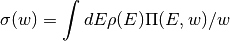
dmft.utils.bubble(A1, A2, nf)¶ Calculates the Polarization Bubble convolution given 2 Spectral functions
It follows the formula
Parameters: - A1 (1D ndarrays, only information in w) – Correspond to the spectral functions
- A2 (1D ndarrays, only information in w) – Correspond to the spectral functions
- nf (ndarray) – Fermi function
-
dmft.utils.dc_conductivity(lat_A1, lat_A2, dnf, w, dosde)
-
dmft.utils.differential_weight(grid)¶ For the grid array calculate the half-way differentials
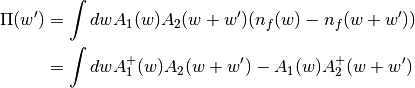
Examples using dmft.utils.differential_weight
-
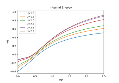
dmft.utils.optical_conductivity(lat_A1, lat_A2, nf, w, dosde)¶ Calculates the optical conductivity from lattice spectral functions
Parameters: - lat_A1 (2D ndarrays) – lattice Spectral functions A(E,w)
- lat_A2 (2D ndarrays) – lattice Spectral functions A(E,w)
- nf (1D ndarray) – fermi function
- w (1D ndarray) – real frequency array
- dosde (1D ndarray) – differentially weighted density of states dE ρ(E)
Returns: - Re σ(w) (1D ndarray)
- Real part of optical conductivity. Posterior scaling required
See also
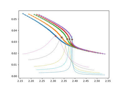
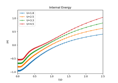
Examples using dmft.utils.optical_conductivity
-
dmft.utils.trapz(y, x=None, dx=1.0, axis=-1)¶ Integrate along the given axis using the composite trapezoidal rule.
Integrate y (x) along given axis.
Parameters: - y (array_like) – Input array to integrate.
- x (array_like, optional) – The sample points corresponding to the y values. If x is None, the sample points are assumed to be evenly spaced dx apart. The default is None.
- dx (scalar, optional) – The spacing between sample points when x is None. The default is 1.
- axis (int, optional) – The axis along which to integrate.
Returns: trapz – Definite integral as approximated by trapezoidal rule.
Return type: See also
sum(),cumsum()Notes
Image [2] illustrates trapezoidal rule – y-axis locations of points will be taken from y array, by default x-axis distances between points will be 1.0, alternatively they can be provided with x array or with dx scalar. Return value will be equal to combined area under the red lines.
References
[1] Wikipedia page: http://en.wikipedia.org/wiki/Trapezoidal_rule [2] Illustration image: http://en.wikipedia.org/wiki/File:Composite_trapezoidal_rule_illustration.png Examples
>>> np.trapz([1,2,3])
4.0
>>> np.trapz([1,2,3], x=[4,6,8])
8.0
>>> np.trapz([1,2,3], dx=2)
8.0
>>> a = np.arange(6).reshape(2, 3)
>>> a
array([[0, 1, 2],
       [3, 4, 5]])
>>> np.trapz(a, axis=0)
array([ 1.5,  2.5,  3.5])
>>> np.trapz(a, axis=1)
array([ 2.,  8.])