Optical conductivity of bonding Spectral Function

# Author: Óscar Nájera

from __future__ import (absolute_import, division, print_function,
                        unicode_literals)

import matplotlib.pyplot as plt
import numpy as np

import dmft.common as gf
import dmft.dimer as dimer
import dmft.ipt_imag as ipt
from dmft.utils import optical_conductivity


def loop_u_tp(u_range, tprange, beta, seed='mott gap'):
    tau, w_n = gf.tau_wn_setup(dict(BETA=beta, N_MATSUBARA=max(5 * beta, 256)))
    giw_d, giw_o = dimer.gf_met(w_n, 0., 0., 0.5, 0.)
    if seed == 'mott gap':
        giw_d, giw_o = 1 / (1j * w_n + 4j / w_n), np.zeros_like(w_n) + 0j

    sigma_iw = []
    for u_int, tp in zip(u_range, tprange):
        giw_d, giw_o, loops = dimer.ipt_dmft_loop(
            beta, u_int, tp, giw_d, giw_o, tau, w_n)
        g0iw_d, g0iw_o = dimer.self_consistency(
            1j * w_n, 1j * giw_d.imag, giw_o.real, 0., tp, 0.25)
        siw_d, siw_o = ipt.dimer_sigma(u_int, tp, g0iw_d, g0iw_o, tau, w_n)
        sigma_iw.append((siw_d.copy(), siw_o.copy()))
        print(seed, ' U', u_int, ' tp: ', tp, ' loops: ', loops)

    return np.array(sigma_iw), w_n


def plot_optical_cond(sigma_iw, ur, tp, w_n, w, w_set, beta, seed):
    nuv = w[w > 0]
    zerofreq = len(nuv)
    dw = w[1] - w[0]
    E = np.linspace(-1, 1, 61)
    dos = np.exp(-2 * E**2) / np.sqrt(np.pi / 2)
    de = E[1] - E[0]
    dosde = (dos * de).reshape(-1, 1)
    nf = gf.fermi_dist(w, beta)
    eta = 0.8

    for U, (sig_d, sig_o) in zip(ur, sigma_iw):
        ss, sa = dimer.pade_diag(sig_d, sig_o, w_n, w_set, w)

        lat_Aa = (-1 / np.add.outer(-E, w + tp + 4e-2j - sa)).imag / np.pi
        lat_As = (-1 / np.add.outer(-E, w - tp + 4e-2j - ss)).imag / np.pi
        #lat_Aa = .5 * (lat_Aa + lat_As)
        #lat_As = lat_Aa

        a = optical_conductivity(lat_Aa, lat_Aa, nf, w, dosde)
        a += optical_conductivity(lat_As, lat_As, nf, w, dosde)
        b = optical_conductivity(lat_Aa, lat_As, nf, w, dosde)
        b += optical_conductivity(lat_As, lat_Aa, nf, w, dosde)

        #b *= tp**2 * eta**2 / 2 / .25

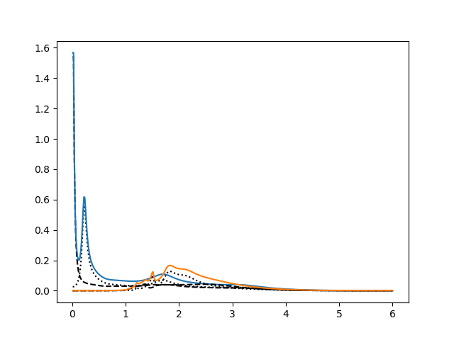
        sigma_E_sum_a = .5 * a[w > 0]
        plt.plot(nuv, sigma_E_sum_a, 'k--')
        sigma_E_sum_i = .5 * b[w > 0]
        plt.plot(nuv, sigma_E_sum_i, 'k:')
        sigma_E_sum = .5 * (a + b)[w > 0]
        plt.plot(nuv, sigma_E_sum)

        # To save data manually at some point
        np.savez('opt_cond{}'.format(seed), nuv=nuv, sigma_E_sum=sigma_E_sum)

        return sigma_E_sum_a, sigma_E_sum_i, sigma_E_sum, nuv

Metals

urange = [2.5]  # [1.5, 2., 2.175, 2.5, 3.]
BETA = 100.
tp = 0.3
w = np.linspace(-6, 6, 800)
w_set = np.concatenate((np.arange(100), np.arange(100, 200, 2)))
sigma_iw, w_n = loop_u_tp(urange, tp * np.ones_like(urange), BETA, "M")

sm_a, sm_i, sm, nuv = plot_optical_cond(
    sigma_iw, urange, tp, w_n, w, w_set, BETA, 'met')

sigma_iw, w_n = loop_u_tp(urange, tp * np.ones_like(urange), BETA)
si_a, si_i, si, nuv = plot_optical_cond(
    sigma_iw, urange, tp, w_n, w, w_set, BETA, 'ins')

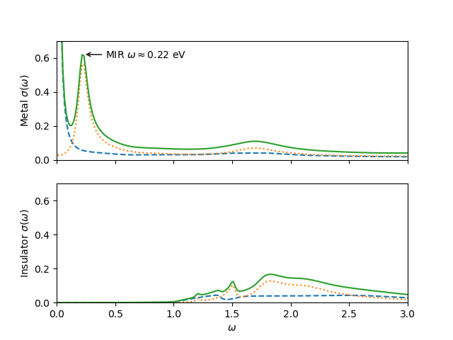
fig, ax = plt.subplots(2, 1, sharex=True, sharey=True)
ax[0].plot(nuv, sm_a, '--')
ax[0].plot(nuv, sm_i, ':')
ax[0].plot(nuv, sm, '-')

ax[1].plot(nuv, si_a, '--')
ax[1].plot(nuv, si_i, ':')
ax[1].plot(nuv, si, '-')
ax[0].set_xlim([0, 3])
ax[0].set_ylim([0, 0.7])

ax[1].set_xlabel(r'$\omega$')
ax[0].set_ylabel(r'Metal $\sigma(\omega)$')
ax[1].set_ylabel(r'Insulator $\sigma(\omega)$')

ax[0].annotate(r"MIR $\omega \approx 0.22$ eV",
               xy=(0.23, 0.62), arrowprops=dict(arrowstyle='->'), xytext=(0.42, 0.6))
plt.savefig('fig_optcond_decomp.pdf', format='pdf',
            transparent=False, bbox_inches='tight', pad_inches=0.05)

• 
• 

Out:

M  U 2.5  tp:  0.3  loops:  85
mott gap  U 2.5  tp:  0.3  loops:  25

Total running time of the script: ( 0 minutes 1.534 seconds)