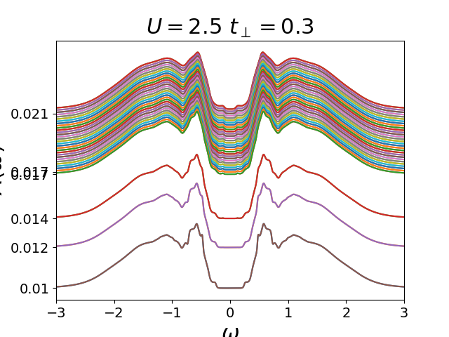
Evolution of DOS as function of temperature

Using a real frequency solver in the IPT scheme the Density of states is tracked through the first orders transition.

# Created Tue Jun 14 15:44:38 2016
# Author: Óscar Nájera

from __future__ import division, absolute_import, print_function

import numpy as np
import scipy.signal as signal
from scipy.integrate import trapz
import matplotlib.pyplot as plt

import dmft.common as gf
import dmft.ipt_real as ipt
from dmft.utils import optical_conductivity


import slaveparticles.quantum.dos as dos

plt.matplotlib.rcParams.update({'axes.labelsize': 22,
                                'xtick.labelsize': 14, 'ytick.labelsize': 14,
                                'axes.titlesize': 22})


def loop_beta(u_int, tp, betarange, seed='mott gap'):
    """Solves IPT dimer and return Im Sigma_AA, Re Simga_AB

    returns list len(betarange) x 2 Sigma arrays
"""

    s = []
    g = []
    w = np.linspace(-6, 6, 2**13)
    dw = w[1] - w[0]
    gss = gf.semi_circle_hiltrans(w + 5e-3j - tp - 1)
    gsa = gf.semi_circle_hiltrans(w + 5e-3j + tp + 1)
    for beta in betarange:
        print('U: ', u_int, 'tp: ', tp, 'Beta', beta)
        nfp = dos.fermi_dist(w, beta)
        (gss, gsa), (ss, sa) = ipt.dimer_dmft(u_int, tp, nfp, w, dw, gss, gsa)
        g.append((gss, gsa))
        s.append((ss, sa))

    return np.array(g), np.array(s)


def simulation(U, tp, betarange):
    try:
        storage = np.load('dimer_Tevol_U{}tp{}.npz'.format(U, tp))
        betarange = storage['betarange']
        gwi = storage['gwi']
        swi = storage['swi']
    except FileNotFoundError:
        gwi, swi = loop_beta(U, tp, betarange)
        np.savez('dimer_Tevol_U{}tp{}.npz'.format(U, tp),
                 betarange=betarange, gwi=gwi, swi=swi)
    return gwi, swi, betarange


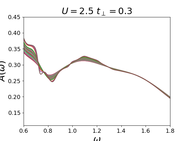
def plot_spectralfunc(gwi, betarange, yshift=False):
    plt.figure()
    shift = 0
    for (gss, gsa), beta in zip(gwi, betarange):
        gloc = .5 * (gss + gsa)
        if yshift:
            shift = 100 / beta
        plt.plot(w, shift - gloc.imag / np.pi)

    plt.xlabel(r'$\omega$')
    plt.ylabel(r'$A(\omega)$')
    plt.xlim([-3, 3])

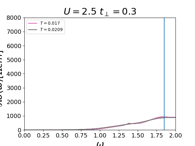
Polarization Bubble and optical conductivity

def optical_cond(ss, sa, tp, w, beta):
    E = np.linspace(-1, 1, 61)
    dos = np.exp(-2 * E**2) / np.sqrt(np.pi / 2)
    de = E[1] - E[0]
    dosde = (dos * de).reshape(-1, 1)
    nf = gf.fermi_dist(w, beta)

    lat_Aa = (-1 / np.add.outer(-E, w + tp - sa)).imag / np.pi
    lat_As = (-1 / np.add.outer(-E, w - tp - ss)).imag / np.pi

    a = optical_conductivity(lat_Aa, lat_Aa, nf, w, dosde)
    b = optical_conductivity(lat_As, lat_As, nf, w, dosde)
    c = optical_conductivity(lat_Aa, lat_As, nf, w, dosde)
    d = optical_conductivity(lat_As, lat_Aa, nf, w, dosde)

    return np.sum((a, b, c, d), axis=0)

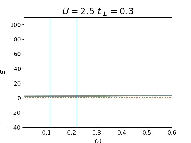
s-SNIM Experiment

def permitivity(real_sig, betarange, unit_weight):
    dw = w[1] - w[0]
    epsilon = []
    for res, beta in zip(real_sig, betarange):
        sig = signal.hilbert(res, len(res) * 4)[:len(res)]
        ep = 1 + 1j * sig / \
            (w - dw / 2) * unit_weight * 0.0074  # final unit conversion in SI
        epsilon.append(ep)
    return epsilon


def plot_epsilon(epsilon, w):
    plt.figure()
    for ep in epsilon:
        plt.plot(w, ep.real, '-', w, ep.imag, ':')
    plt.xlabel(r'$\omega$')
    plt.ylabel(r'$\varepsilon$')


def aal_ef(eps_sample, t, e_tip=-1300 + 960j, a=20):
    beta = (eps_sample - 1) / (eps_sample + 1)
    alpha = 4 * np.pi * a ** 3 * (e_tip - 1) / (e_tip + 2)
    return alpha * (1 + beta) / (1 - alpha * beta / (16 * np.pi * (3 * a + 2 * a * np.cos(t))**3))

Spectral function Dispersion

# eps_k = np.linspace(-1., 1., 61)

# ss, sa = swi[18]
# lat_gfs = 1 / np.add.outer(-eps_k, w - tp + 5e-2j - ss)
# lat_gfa = 1 / np.add.outer(-eps_k, w + tp + 5e-2j - sa)
# Aw = np.clip(-.5 * (lat_gfa + lat_gfs).imag / np.pi, 0, 8)
# plot_band_dispersion(w, Aw, 'Local ', eps_k, 'intensity')
# plot_band_dispersion(w, -lat_gfa.imag / np.pi, 'Local ', eps_k, 'intensity')
# plt.ylim([-3, 3])

w = np.linspace(-6, 6, 2**13)
t = np.linspace(-np.pi, np.pi, 600)
cos2 = np.cos(2 * t)

# Reference insulator data from http://dx.doi.org/10.1126/science.1150124
s_ins = np.loadtxt(
    '/home/oscar/Dropbox/org/phd/dimer_lattice/optical conductivity/ins_340.csv', comments='x', delimiter=',').T
s_exp_weight = trapz(s_ins[1], x=s_ins[0] / 8056.54)

U = 2.8 tp = 0.3 higb = np.array([100., 70., 60., 50.]) temp = np.linspace(0.023, 0.035, 30)

sig_wei = 20

U = 2.5
tp = 0.3
higb = np.array([100., 80., 70.])
temp = np.linspace(0.017, 0.021, 30)
sig_wei = 3

temp = np.linspace(0.04, 0.05, 30) temp = np.linspace(0.023, 0.035, 30)

betarange = np.concatenate((higb, 1 / temp, 1 / temp[::-1], higb[::-1]))

gwi, swi, betarange = simulation(U, tp, betarange)
resi = [optical_cond(ss, sa, tp, w, beta)
        for (ss, sa), beta in zip(swi, betarange)]

Plots

temp_set = [0, 1, 2, 3, 4, len(temp)]
plot_spectralfunc(gwi, betarange, yshift=True)
plt.yticks(100 / betarange[temp_set], np.around(1 / betarange, 3)[temp_set])
plt.title(r'$U={}$ $t_\perp={}$'.format(U, tp))
plt.savefig('dimer_sig_Tevo_U{}tp{}_iptre_yshift.pdf'.format(U, tp))

plot_spectralfunc(gwi, betarange, yshift=False)
plt.title(r'$U={}$ $t_\perp={}$'.format(U, tp))
plt.savefig('dimer_dos_Tevo_U{}tp{}_iptre_ontop.pdf'.format(U, tp))
plt.xlim([-.6, .6])
plt.ylim([0, 0.11])
plt.savefig('dimer_dos_Tevo_U{}tp{}_iptre_gapzoom.pdf'.format(U, tp))
plt.xlim([.6, 1.8])
plt.ylim([0.11, 0.45])
plt.savefig('dimer_dos_Tevo_U{}tp{}_iptre_qp_zoom.pdf'.format(U, tp))

rdw = (w > 0) * (w < s_ins[0][-1] / 8056.54)
sim_weight = trapz(resi[sig_wei][rdw], x=w[rdw])
unit_weight = s_exp_weight / sim_weight

plt.figure()
for res, beta in zip(resi, betarange):
    plt.plot(w, unit_weight * res)

plt.plot(w, unit_weight * resi[sig_wei], lw=2,
         label=r'$T={:.3}$'.format(1 / betarange[sig_wei]))
plt.plot(w, unit_weight * resi[len(temp) + 1], lw=2,
         label=r'$T={:.3}$'.format(1 / betarange[len(temp) + 1]))
plt.xlabel(r'$\omega$')
plt.ylabel(r'$\Re \sigma(\omega)[\Omega cm]^{-1}$')
plt.axvline(s_ins[0][-1] / 8056.54)
plt.ylim([0, 8000])
plt.xlim([0, 2])
plt.legend(loc=0)
plt.title(r'$U={}$ $t_\perp={}$'.format(U, tp))
plt.savefig('dimer_resigma_Tevo_U{}tp{}_iptre.pdf'.format(U, tp))

epsilon = permitivity(resi, betarange, unit_weight)
plot_epsilon(epsilon, w)
plt.axvline(w[4174])
plt.axvline(w[4247])
plt.ylim([-40, 110])
#plt.ylim([-1, 10])
plt.xlim([0.01, .6])
plt.title(r'$U={}$ $t_\perp={}$'.format(U, tp))
plt.savefig('dimer_epsilon_Tevo_U{}tp{}_iptre.pdf'.format(U, tp))

• 
• 
• 
• 

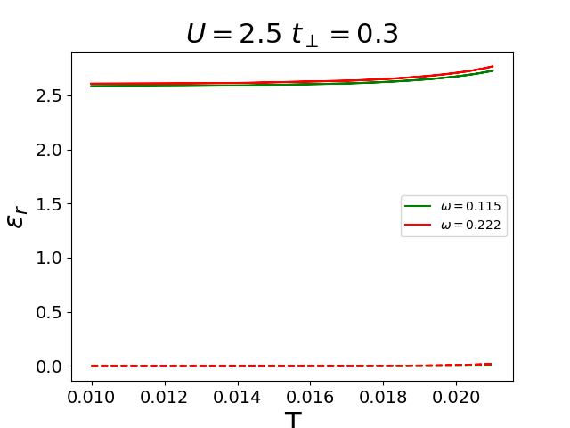
plt.figure()
epr = np.array([ep[4174] for ep in epsilon])
epp = np.array([ep[4247] for ep in epsilon])
plt.plot(1 / betarange, epr.real, 'g', label=r'$\omega=0.115$')
plt.plot(1 / betarange, epr.imag, "g--")
plt.plot(1 / betarange, epp.real, 'r', label=r'$\omega=0.222$')
plt.plot(1 / betarange, epp.imag, "r--")
plt.xlabel('T')
plt.ylabel(r'$\varepsilon_r$')
plt.legend(loc=0)
plt.title(r'$U={}$ $t_\perp={}$'.format(U, tp))
plt.savefig('dimer_epsilon_Tevo_U{}tp{}_iptre_fixfreq.pdf'.format(U, tp))

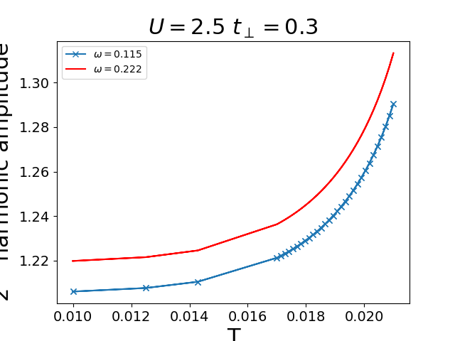
# This normalization because this is an intensity measure so just to have
# readable numbers
sam = np.array([abs(trapz(aal_ef(ep, t) * cos2, t)) for ep in epr]) / 1e4
sap = np.array([abs(trapz(aal_ef(ep, t) * cos2, t, -474.41 + 248.61j))
                for ep in epp]) / 1e4

plt.figure()
plt.plot(1 / betarange, sam, 'x-', label=r'$\omega=0.115$')
plt.plot(1 / betarange, sap, 'r', label=r'$\omega=0.222$')
plt.xlabel('T')
plt.ylabel('2$^{nd}$ harmonic amplitude')
plt.title(r'$U={}$ $t_\perp={}$'.format(U, tp))
plt.legend(loc=0)
plt.savefig('dimer_s2_Tevo_U{}tp{}_iptre_fixfreq.pdf'.format(U, tp))

Total running time of the script: ( 0 minutes 57.246 seconds)