Landau Theory of the Mott transition

Perform a fit of the order parameter, linked to double occupation to match a Landau theory formulation in correspondence to Kotliar, G., Lange, E., & Rozenberg, M. J. (2000). Landau Theory of the Finite Temperature Mott Transition. Phys. Rev. Lett., 84(22), 5180–5183. http://dx.doi.org/10.1103/PhysRevLett.84.5180

Warning

Not reproduced for the moment

from scipy.optimize import curve_fit
import numpy as np
import matplotlib.pyplot as plt
from mpl_toolkits.mplot3d import axes3d
import dmft.dimer as dimer
import dmft.common as gf
import dmft.ipt_imag as ipt
from dmft.utils import differential_weight as diff


def extract_double_occupation(beta, u_range):
    docc = []
    tau, w_n = gf.tau_wn_setup(dict(BETA=beta, N_MATSUBARA=beta))
    g_iwn = gf.greenF(w_n)
    for u_int in u_range:
        g_iwn, sigma = ipt.dmft_loop(u_int, 0.5, g_iwn, w_n, tau, conv=1e-4)
        docc.append(ipt.epot(g_iwn, sigma, u_int, beta, w_n) * 2 / u_int)
    return np.array(docc)


# calculating multiple regions
fac = np.arctan(.15 * np.sqrt(3) / .10)
udelta = np.tan(np.linspace(-fac, fac, 91)) * .10 / np.sqrt(3)
dudelta = diff(udelta)
data = []
bet_uc = [(18, 2.312),
          (19, 2.339),
          (20, 2.3638),
          (20.5, 2.375),
          (21, 2.386)]

for beta, uc in bet_uc:
    urange = udelta + uc + .07
    data.append(extract_double_occupation(beta, urange) - 0.003)

plt.figure()
bc = [b for b, _ in bet_uc]
d_c = [dc[int(len(udelta) / 2)] for dc in data]
for dd, dc, (beta, uc) in zip(data, d_c, bet_uc):
    plt.plot(uc + udelta, dd, '+-', label=beta)

plt.plot([uc for _, uc in bet_uc], [dc[45] for dc in data], 'o')

for dd, (beta, uc) in zip(data, bet_uc):
    chi = diff(dd) / dudelta
    plt.plot(uc + udelta, chi / np.min(chi) * .035, ':')

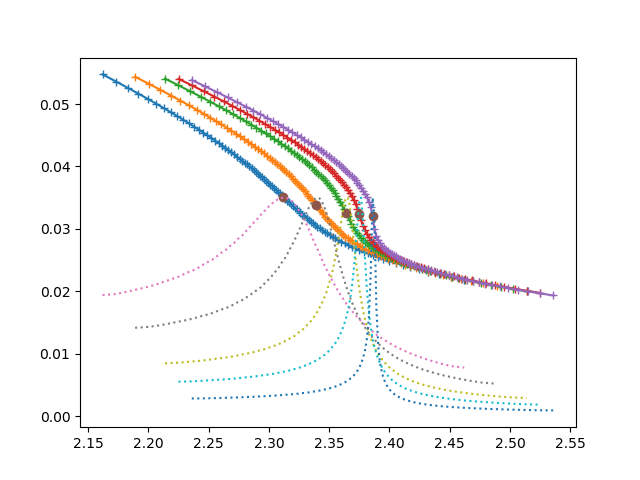
effective scaling

plt.close()
plt.figure()
d_c = [dc[45] for dc in data]
for dd, dc, (beta, uc) in zip(data, d_c, bet_uc):
    plt.plot(udelta, dd - dc, lw=2)


def fit_cube(eta, c):
    return c * eta**3


plt.gca().set_color_cycle(None)
for dd, dc, (beta, uc) in zip(data, d_c, bet_uc):
    rd = dd - dc
    bound = 35
    popt, pcov = curve_fit(fit_cube, rd[bound:-bound], udelta[bound:-bound])
    ft = fit_cube(rd, *popt)
    plt.plot(ft, rd)
    print(popt)

plt.xlim([-.15, .15])

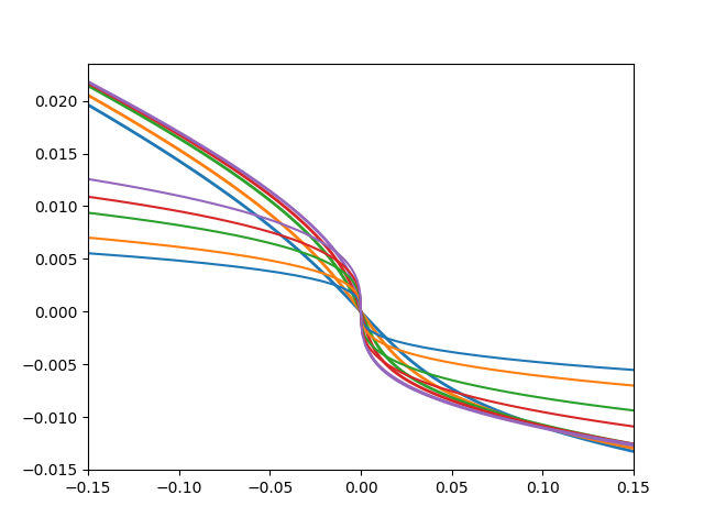
Out:

[-883505.67162143]
[-433371.7767214]
[-181617.47843594]
[-115684.11364568]
[-75369.81958888]

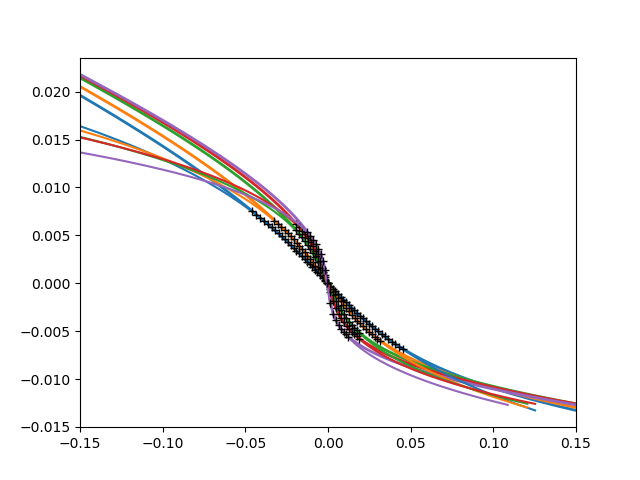
cubic + linear

def fit_cube_lin(eta, c, p):
    return c * eta**3 + p * eta


for dd, dc, (beta, uc) in zip(data, d_c, bet_uc):
    plt.plot(udelta, dd - dc, lw=2)

plt.gca().set_color_cycle(None)
bb = [23, 27, 33, 33, 36]
for dd, dc, bound, (beta, uc) in zip(data, d_c, bb, bet_uc):
    rd = dd - dc
    popt, pcov = curve_fit(
        fit_cube_lin, rd[bound:-bound], udelta[bound:-bound])
    ft = fit_cube_lin(rd, *popt)
    plt.plot(ft, rd)
    plt.plot(ft[bound:-bound], rd[bound:-bound], "k+")
    print(popt)

plt.xlim([-.15, .15])

Out:

[ -1.58437153e+04  -5.47851818e+00]
[ -2.33585353e+04  -4.13738189e+00]
[ -3.49190705e+04  -2.56748085e+00]
[ -4.06160512e+04  -1.72641946e+00]
[ -4.72383167e+04  -8.18454025e-01]

cubic + linear over constant + linear

plt.figure()


def fit_cube_lin(eta, c, p, q, s):
    return (c * eta**3 + p * eta + s) / (1 + q * eta)


for dd, dc, (beta, uc) in zip(data, d_c, bet_uc):
    plt.plot(udelta, dd - dc, lw=2)

plt.gca().set_color_cycle(None)
bb = [20, 26, 33, 33, 37]
for dd, dc, bound, (beta, uc) in zip(data, d_c, bb, bet_uc):
    rd = dd - dc
    popt, pcov = curve_fit(
        fit_cube_lin, rd[bound:-bound], udelta[bound:-bound], p0=[4e4, 0, 3, -.3])
    ft = fit_cube_lin(rd, *popt)
    plt.plot(ft, rd)
    plt.plot(ft[bound:-bound], rd[bound:-bound], "k+")
    print(popt)

plt.xlim([-.15, .15])

Out:

[ -1.76916299e+04  -5.43951224e+00   7.17823742e+00  -2.33400113e-04]
[ -2.54066727e+04  -4.09444802e+00   7.85502769e+00  -2.50641838e-04]
[ -3.73436918e+04  -2.52439784e+00   9.64561095e+00  -2.37444323e-04]
[ -4.29143927e+04  -1.67288401e+00   1.20974775e+01  -5.19144949e-04]
[ -5.15225117e+04  -7.30668859e-01  -3.81150442e+00  -7.46327101e-04]

Beta 21 study

def fitchi(urange, a, uc, x0):
    return a * np.abs(urange - uc)**(-2 / 3) + x0


ulim = 44
popt, pcov = curve_fit(fitchi, urange[:ulim], chi[
                       :ulim], p0=[-0.01, 2.391, -0.01])
ft = fitchi(urange, *popt)
plt.plot(urange, ft)
plt.plot(urange[:ulim], ft[:ulim], lw=2)
print(popt)

ulim += 4
popt, pcov = curve_fit(
    fitchi, urange[ulim:], chi[ulim:], p0=[-0.01, 2.391, 0])
ft = fitchi(urange, *popt)
plt.plot(urange, ft)
plt.plot(urange[ulim:], ft[ulim:], lw=2)
print(popt)

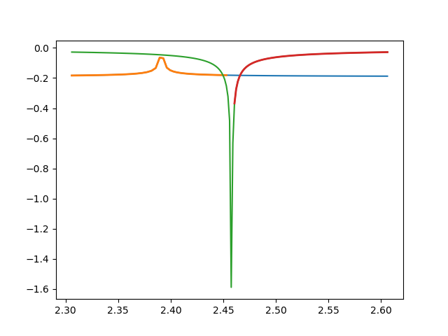
Out:

[  1.82409742e-03   2.39121666e+00  -1.92832349e-01]
[-0.00724163  2.45785292 -0.00253954]

Total running time of the script: ( 0 minutes 5.079 seconds)