IPT Solver Existence of Metalic and insulating solution¶

Within the iterative perturbative theory (IPT) the aim is to express the self-energy of the impurity problem as

$\Sigma(\tau) \approx U^2 \mathcal{G}^0(\tau)^3$

the contribution of the Hartree-term is not included here as it is cancelled

from __future__ import division, absolute_import, print_function

import numpy as np
import matplotlib.pylab as plt


from dmft.ipt_imag import dmft_loop
from dmft.common import greenF, tau_wn_setup, pade_continuation, fermi_dist
from dmft.utils import optical_conductivity

U = 2.7
BETA = 100.
tau, w_n = tau_wn_setup(dict(BETA=BETA, N_MATSUBARA=2**9))
omega = np.linspace(-4, 4, 600)
eps_k = np.linspace(-1, 1, 61)
dos = np.exp(-2 * eps_k**2) / np.sqrt(np.pi / 2)
de = eps_k[1] - eps_k[0]
dosde = (dos * de).reshape(-1, 1)
nf = fermi_dist(omega, BETA)

Insulator Calculations¶

ig_iwn, is_iwn = dmft_loop(
    U, 0.5, -1.j / (w_n - 1 / w_n), w_n, tau, conv=1e-12)
igw = pade_continuation(ig_iwn, w_n, omega, np.arange(100))
isigma_w = pade_continuation(is_iwn, w_n, omega, np.arange(100))
lat_gf = 1 / (np.add.outer(-eps_k, omega + 4e-2j) - isigma_w)
lat_Aw = -lat_gf.imag / np.pi
icond = optical_conductivity(lat_Aw, lat_Aw, nf, omega, dosde)

Metal Calculations¶

mg_iwn, s_iwn = dmft_loop(U, 0.5, greenF(w_n), w_n, tau, conv=1e-10)
mgw = pade_continuation(mg_iwn, w_n, omega, np.arange(100))
msigma_w = omega - 0.25 * mgw - 1 / mgw
lat_gf = 1 / (np.add.outer(-eps_k, omega + 4e-2j) - msigma_w)
lat_Aw = -lat_gf.imag / np.pi
mcond = optical_conductivity(lat_Aw, lat_Aw, nf, omega, dosde)

Plots¶

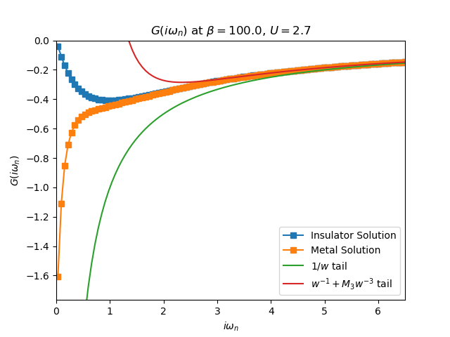
fig_giw, giw_ax = plt.subplots()
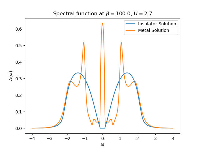
fig_gw, gw_ax = plt.subplots()
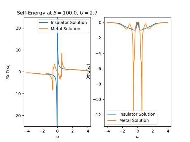
fig_sw, sw_ax = plt.subplots(1, 2, sharex=True)
fig_cond, cond_ax = plt.subplots()

giw_ax.plot(w_n, ig_iwn.imag, 's-', label='Insulator Solution')
gw_ax.plot(omega, -igw.imag / np.pi, label='Insulator Solution')
sw_ax[0].plot(omega, isigma_w.real, label='Insulator Solution')
sw_ax[1].plot(omega, isigma_w.imag, label='Insulator Solution')
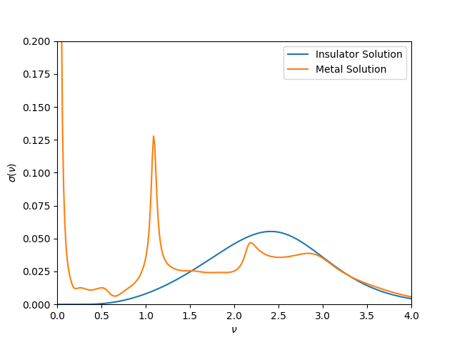
cond_ax.plot(omega, icond, label='Insulator Solution')
giw_ax.plot(w_n, mg_iwn.imag, 's-', label='Metal Solution')
gw_ax.plot(omega, -mgw.imag / np.pi, label='Metal Solution')
sw_ax[0].plot(omega, msigma_w.real, label='Metal Solution')
sw_ax[1].plot(omega, msigma_w.imag, label='Metal Solution')
cond_ax.plot(omega, mcond, label='Metal Solution')

giw_ax.plot(w_n, -1 / w_n, label='$1/w$ tail')
giw_ax.plot(w_n, -1 / w_n + U**2 / 4 / w_n**3,
            label='$w^{-1} + M_3 w^{-3}$ tail')

cut = int(6.5 * BETA / np.pi)
giw_ax.set_xlim([0, 6.5])
giw_ax.set_ylim([mg_iwn.imag.min() * 1.1, 0])

giw_ax.set_ylabel(r'$G(i\omega_n)$')
giw_ax.set_xlabel(r'$i\omega_n$')
giw_ax.set_title(r'$G(i\omega_n)$ at $\beta= {}$, $U= {}$'.format(BETA, U))
giw_ax.legend(loc=0)

gw_ax.set_ylabel(r'$A(\omega)$')
gw_ax.set_xlabel(r'$\omega$')
gw_ax.set_title(r'Spectral function at $\beta= {}$, $U= {}$'.format(BETA, U))
gw_ax.legend(loc=0)

sw_ax[0].set_ylabel(r'$\Re e \Sigma(\omega)$')
sw_ax[0].set_ylim([-25, 25])
sw_ax[1].set_ylabel(r'$\Im m \Sigma(\omega)$')
sw_ax[0].set_xlabel(r'$\omega$')
sw_ax[1].set_xlabel(r'$\omega$')
sw_ax[0].set_title(r'Self-Energy at $\beta= {}$, $U= {}$'.format(BETA, U))
sw_ax[0].legend(loc=0)
sw_ax[1].legend(loc=0)

cond_ax.legend(loc=0)
cond_ax.set_xlabel(r'$\nu$')
cond_ax.set_ylabel(r'$\sigma(\nu)$')
cond_ax.set_ylim([0, .2])
cond_ax.set_xlim([0, 4])