Isolated molecule spectral function
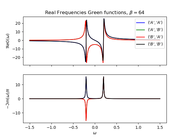
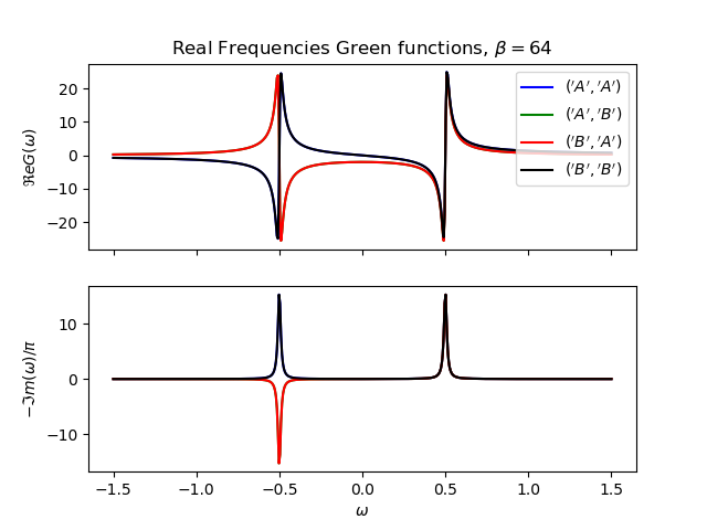
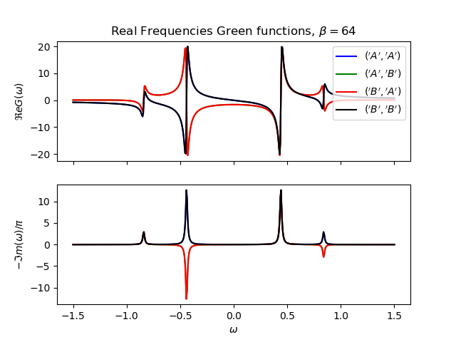
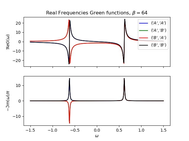
For the case of contact interaction in the di-atomic molecule case spectral function are evaluated by means of the Lehmann representation
# author: Óscar Nájera

from __future__ import division, absolute_import, print_function
from itertools import product
import matplotlib.pyplot as plt
import numpy as np
import scipy.linalg as LA
from dmft.common import matsubara_freq, gw_invfouriertrans
import dmft.dimer as dimer
import slaveparticles.quantum.operators as op
Real space representation
def plot_real_gf(eig_e, eig_v, oper_pair, c_v, names, beta):
_, axw = plt.subplots(2, sharex=True)
w = np.linspace(-1.5, 1.5, 500) + 1j * 1e-2
gfs = [op.gf_lehmann(eig_e, eig_v, c.T, beta, w, d) for c, d in oper_pair]
for gw, color, name in zip(gfs, c_v, names):
axw[0].plot(w.real, gw.real, color, label=r'${}$'.format(name))
axw[1].plot(w.real, -1 * gw.imag / np.pi, color)
axw[0].legend()
axw[0].set_title(
r'Real Frequencies Green functions, $\beta={}$'.format(beta))
axw[0].set_ylabel(r'$\Re e G(\omega)$')
axw[1].set_ylabel(r'$-\Im m(\omega)/\pi$')
axw[1].set_xlabel(r'$\omega$')
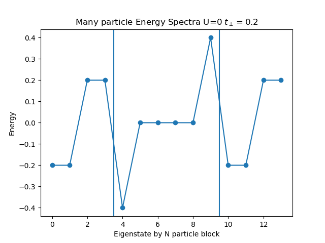
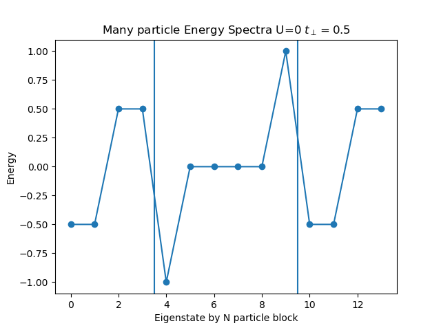
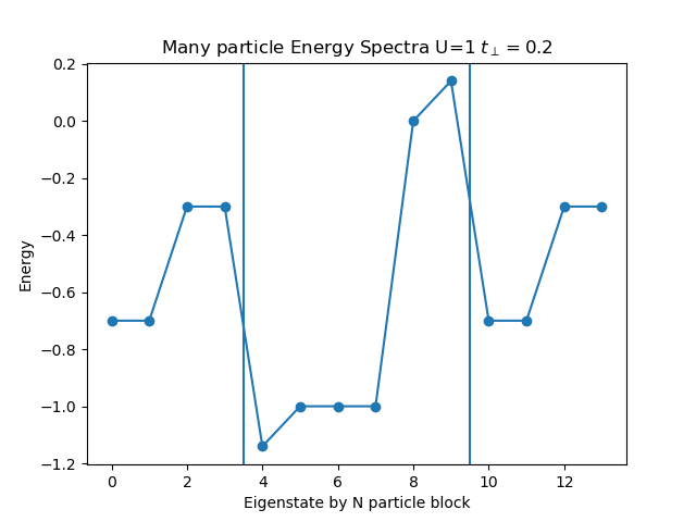
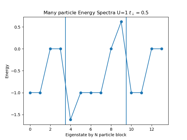
def plot_eigen_spectra(U, mu, tp):
h_at, oper = dimer.hamiltonian(U, mu, tp)
eig_e = []
eig_e.append(LA.eigvalsh(h_at[1:5, 1:5].todense()))
eig_e.append(LA.eigvalsh(h_at[5:11, 5:11].todense()))
eig_e.append(LA.eigvalsh(h_at[11:15, 11:15].todense()))
plt.figure()
plt.title('Many particle Energy Spectra U={} $t_\perp={}$'.format(U, tp))
plt.plot(np.concatenate(eig_e), "o-")
plt.ylabel('Energy')
plt.xlabel('Eigenstate by N particle block')
plt.axvline(x=3.5)
plt.axvline(x=9.5)
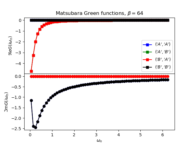
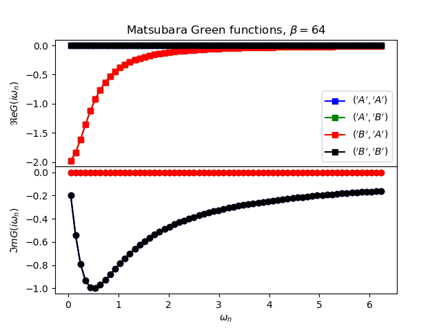
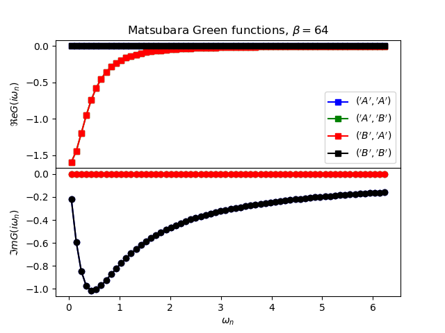
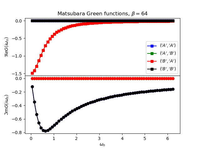
def plot_matsubara_gf(eig_e, eig_v, oper_pair, c_v, names, beta, U, mu, tp):
gwp, axwn = plt.subplots(2, sharex=True)
gwp.subplots_adjust(hspace=0)
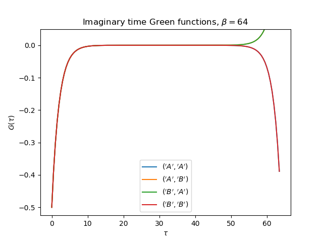
gtp, axt = plt.subplots()
wn = matsubara_freq(beta, beta)
tau = np.arange(0, beta, .5)
gfs = [op.gf_lehmann(eig_e, eig_v, c.T, beta, 1j * wn, d)
for c, d in oper_pair]
for giw, color, name in zip(gfs, c_v, names):
axwn[0].plot(wn, giw.real, color + 's-', label=r'${}$'.format(name))
axwn[1].plot(wn, giw.imag, color + 'o-')
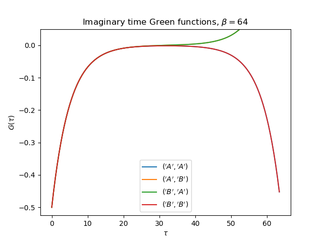
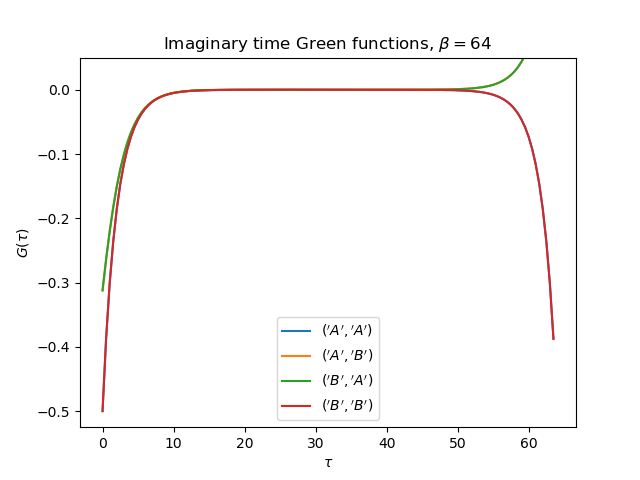
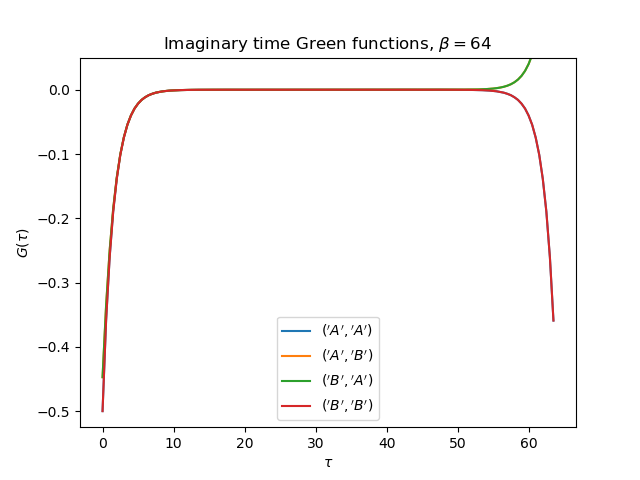
tail = [0., tp, 0.] if name[0] != name[1] else [1., 0., U**2 / 4.]
gt = gw_invfouriertrans(giw, tau, wn, tail)
axt.plot(tau, gt, label=r'${}$'.format(name))
axwn[0].legend()
axwn[0].set_title(
r'Matsubara Green functions, $\beta={}$'.format(beta))
axwn[1].set_xlabel(r'$\omega_n$')
axwn[0].set_ylabel(r'$\Re e G(i\omega_n)$')
axwn[1].set_ylabel(r'$\Im m G(i\omega_n)$')
axt.set_ylim(top=0.05)
axt.legend(loc=0)
axt.set_title(
r'Imaginary time Green functions, $\beta={}$'.format(beta))
axt.set_xlabel(r'$\tau$')
axt.set_ylabel(r'$G(\tau)$')
def plot_greenfunctions(beta, U, mu, tp):
c_v = ['b', 'g', 'r', 'k']
names = [r'a\uparrow', r'a\downarrow', r'b\uparrow', r'b\downarrow']
plot_eigen_spectra(U, mu, tp)
h_at, oper = dimer.hamiltonian(U, mu, tp)
oper_pair = list(product([oper[0], oper[1]], repeat=2))
names = list(product('AB', repeat=2))
eig_e, eig_v = op.diagonalize(h_at.todense())
plot_real_gf(eig_e, eig_v, oper_pair, c_v, names, beta)
plot_matsubara_gf(eig_e, eig_v, oper_pair, c_v, names, beta, U, mu, tp)
The symmetric and anti-symmetric bands
#h_at, oper = dimer.hamiltonian_diag(U, mu, tp)
#eig_e, eig_v = op.diagonalize(h_at.todense())
#
#oper_pair = product([oper[0], oper[1]], repeat=2)

#plot_real_gf(eig_e, eig_v, oper_pair, c_v, names)

# TODO: verify the asy/sym basis scale
# TODO: view in the local one the of diag terms
Total running time of the script: ( 0 minutes 2.946 seconds)