Landau Theory of the Mott transition¶

Perform a fit of the order parameter, linked to double occupation to match a Landau theory formulation in correspondence to Kotliar, G., Lange, E., & Rozenberg, M. J. (2000). Landau Theory of the Finite Temperature Mott Transition. Phys. Rev. Lett., 84(22), 5180–5183. http://dx.doi.org/10.1103/PhysRevLett.84.5180

Study above the critical point

Out:

[67 61 62 61 59 57 55 53 51 49 47 45 44 42 41 39 38 37 37 37 38 38 38 39 39
39 39 39 40 40 40 40 40 40 40 40 41 41 41 41 41 41 41 41 41 41 42 42 42
42 42 42 42 42 42 42 43 43 43 43 43 43 43 43 43 43 44 44 44 44 44 44 44
44 44 45 45 45 45 45 45 45 45 45 45 45 45 45 45 45 45 45 45 45 45 45 44
44 43 43 42 42 41 40 39 38 37 36 35 33 32 30 28 27 25 23 21]
[68 64 66 67 66 65 64 62 60 58 56 54 52 50 49 47 46 44 43 42 42 43 43 44 44
45 46 46 47 47 48 48 49 49 49 50 50 51 51 51 52 52 53 53 53 54 54 54 55
55 56 56 56 57 57 57 58 58 58 59 59 59 59 60 60 60 60 61 61 61 61 61 62
62 62 62 62 62 62 62 62 61 61 61 61 60 60 59 59 58 57 57 56 55 54 53 52
49 48 47 45 44 42 41 39 38 36 34 33 31 29 28 26 24 22 21 19]
[67 64 68 70 71 71 71 70 68 67 65 63 61 59 58 56 54 53 51 50 48 47 47 49 49
51 52 53 54 55 56 57 58 60 61 62 63 64 65 66 67 68 70 71 72 73 75 76 77
80 81 82 83 85 86 87 88 89 90 91 92 93 94 95 95 95 96 96 95 95 94 94 93
91 89 88 86 84 83 81 79 77 75 73 71 69 67 65 63 61 59 57 55 53 51 50 48
45 43 41 40 38 37 35 34 32 31 30 28 27 25 24 23 21 20 18 17]
[ 67  64  68  71  72  73  73  73  72  71  69  68  66  64  63  61  59  58
54  53  51  50  49  51  52  53  54  56  57  58  60  61  62  64  66
69  70  72  74  76  78  80  82  84  86  89  91  94  97  99 102 105
111 113 116 119 122 124 126 127 128 129 129 129 127 126 124 121 118
111 108 104 100  97  93  89  86  83  80  77  74  71  69  66  64  61
57  55  53  51  50  48  46  45  43  42  40  39  37  36  35  33  32
30  28  27  26  25  24  22  21  20  19  17  16]
[ 65  63  67  70  73  74  75  76  75  75  74  72  71  70  68  67  65  63
60  59  57  56  54  53  52  53  54  55  57  58  60  61  63  65  67
71  73  75  78  80  83  86  89  92  96 100 104 109 114 120 126 132
147 155 164 172 180 187 193 195 195 192 185 177 168 158 148 139 130
114 108 102  96  91  87  83  79  75  72  69  66  63  61  59  57  55
51  49  47  46  44  43  41  40  39  37  36  35  34  33  32  31  29
27  26  25  24  23  22  21  20  19  18  17  15]
[ 63  61  65  69  72  74  76  77  77  77  77  76  75  74  73  72  71  69
66  65  64  62  61  60  58  57  56  55  55  56  57  59  61  63  65
69  71  73  76  79  82  85  88  92  97 102 107 113 120 129 139 150
182 204 233 270 316 364 387 363 313 262 222 191 168 149 135 123 113
98  92  86  81  77  73  70  67  64  62  59  57  55  53  51  49  48
45  43  42  41  39  38  37  36  35  34  33  32  31  30  29  28  27
25  24  24  23  22  21  20  19  18  17  16  15]
[ 63  60  65  69  72  74  76  77  78  78  78  78  77  76  75  74  73  71
69  67  66  65  63  62  61  60  58  57  56  55  57  58  60  61  63
67  69  72  74  77  80  83  87  91  95 100 106 112 120 129 140 153
191 222 266 336 454 604 554 393 290 229 191 164 144 129 118 108 100
87  82  78  74  70  67  64  62  59  57  55  53  51  49  48  46  45
42  41  40  39  38  36  35  34  33  33  32  31  30  29  28  27  26
25  24  23  22  21  20  19  19  18  17  16  15]
[ -3.86528847e+04  -2.47024433e+01   1.76230198e+01  -6.76142889e-04]
[ -5.66140107e+04  -1.90645920e+01   6.03415912e+00  -1.03353073e-04]
[ -9.29427951e+04  -1.32890339e+01   1.65847125e+00  -2.43110956e-04]
[ -1.25002557e+05  -1.01922703e+01  -3.05401520e-01  -1.92401678e-04]
[ -1.58468430e+05  -7.01333087e+00   1.42348154e+00  -3.21099956e-04]
[ -1.93447631e+05  -3.76601834e+00   9.68173850e+00  -5.89656130e-04]
[ -2.14218382e+05  -2.43545432e+00   4.22759934e+01  -4.49653695e-04]

from scipy.optimize import curve_fit
import numpy as np
import matplotlib.pyplot as plt
import dmft.dimer as dimer
import dmft.common as gf
import dmft.ipt_imag as ipt


def loop_u_tp(u_range, tprange, beta, seed='mott gap'):
    tau, w_n = gf.tau_wn_setup(dict(BETA=beta, N_MATSUBARA=256))
    giw_d, giw_o = dimer.gf_met(w_n, 0., 0., 0.5, 0.)
    if seed == 'ins':
        giw_d, giw_o = 1 / (1j * w_n + 4j / w_n), np.zeros_like(w_n) + 0j

    giw_s = []
    sigma_iw = []
    ekin, epot = [], []
    iterations = []
    for u_int, tp in zip(u_range, tprange):
        giw_d, giw_o, loops = dimer.ipt_dmft_loop(
            beta, u_int, tp, giw_d, giw_o, tau, w_n)
        giw_s.append((giw_d, giw_o))
        iterations.append(loops)
        g0iw_d, g0iw_o = dimer.self_consistency(
            1j * w_n, 1j * giw_d.imag, giw_o.real, 0., tp, 0.25)
        siw_d, siw_o = ipt.dimer_sigma(u_int, tp, g0iw_d, g0iw_o, tau, w_n)
        sigma_iw.append((siw_d.copy(), siw_o.copy()))

        ekin.append(dimer.ekin(giw_d, giw_o, w_n, tp, beta))

        epot.append(dimer.epot(giw_d, w_n, beta, u_int **
                               2 / 4 + tp**2, ekin[-1], u_int))
    print(np.array(iterations))
    # last division in energies because I want per spin epot
    return np.array(giw_s), np.array(sigma_iw), np.array(ekin) / 4, np.array(epot) / 4, w_n


# calculating multiple regions
fac = np.arctan(.55 * np.sqrt(3) / .15)
udelta = np.tan(np.linspace(-fac, fac, 121)) * .15 / np.sqrt(3)
dudelta = np.diff(udelta)
bet_uc = [(18, 3.312),
          (19, 3.258),
          (20, 3.214),
          (20.5, 3.193),
          (21, 3.17),
          (21.5, 3.1467),
          (21.7, 3.138)]

data = []
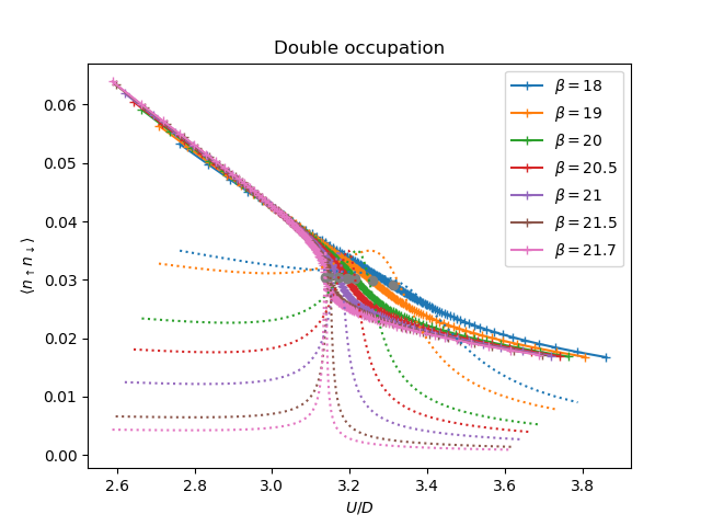
for beta, uc in bet_uc:
    urange = udelta + uc + .07
    giw_s, sigma_iw, ekin, epot, w_n = loop_u_tp(
        urange, .3 * np.ones_like(urange), beta, 'met')
    data.append(2 * epot / urange - 0.003)

plt.figure()
bc = [b for b, _ in bet_uc]
d_c = [dc[int(len(udelta) / 2)] for dc in data]
for dd, dc, (beta, uc) in zip(data, d_c, bet_uc):
    plt.plot(uc + udelta, dd, '+-', label=r'$\beta={}$'.format(beta))

plt.plot([uc for _, uc in bet_uc], d_c, 'o')

plt.gca().set_color_cycle(None)
for dd, (beta, uc) in zip(data, bet_uc):
    chi = np.diff(dd) / dudelta
    plt.plot(uc + udelta[:-1], chi / np.min(chi) * .035, ':')

plt.title(r'Double occupation')
plt.ylabel(r'$\langle n_\uparrow n_\downarrow \rangle$')
plt.xlabel(r'$U/D$')
plt.legend()
plt.savefig("dimer_tp0.3_docc.pdf",
            transparent=False, bbox_inches='tight', pad_inches=0.05)

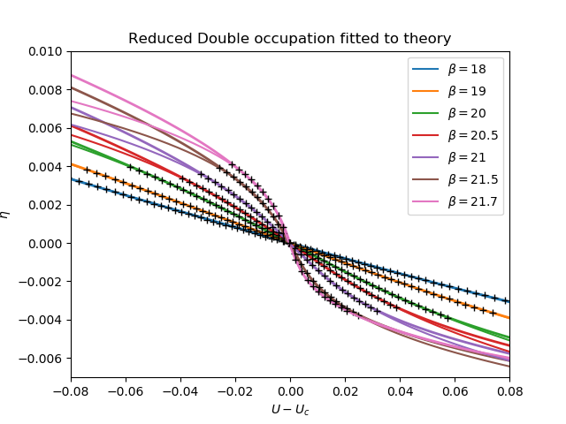
# effective scaling
# cubic + linear over constant + linear


def fit_cube_lin(eta, c, p, q, s):
    return (c * eta**3 + p * eta + s) / (1 + q * eta)


plt.figure()
for dd, dc, (beta, uc) in zip(data, d_c, bet_uc):
    plt.plot(udelta, dd - dc, lw=2)

plt.gca().set_color_cycle(None)
bb = [10, 30, 35, 42, 45, 48, 50]
fits = []
for dd, dc, bound, (beta, uc) in zip(data, d_c, bb, bet_uc):
    rd = dd - dc
    popt, pcov = curve_fit(
        fit_cube_lin, rd[bound:-bound], udelta[bound:-bound], p0=[-4e4, -3, 3, 1])
    fits.append((popt, pcov))
    ft = fit_cube_lin(rd, *popt)
    plt.plot(ft, rd, label=r'$\beta={}$'.format(beta))
    plt.plot(ft[bound:-bound], rd[bound:-bound], "k+")
    print(popt)

plt.xlim([-.08, .08])
plt.ylim([-.007, .01])

plt.title(r'Reduced Double occupation fitted to theory')
plt.ylabel(r'$\eta$')
plt.xlabel(r'$U-U_c$')
plt.legend()
plt.savefig("dimer_tp0.3_eta_landau.pdf",
            transparent=False, bbox_inches='tight', pad_inches=0.05)

Total running time of the script: ( 1 minutes 17.737 seconds)

Generated by Sphinx-Gallery

Landau Theory of the Mott transition¶

Previous topic

Next topic

This Page