Dispersion of the spectral function

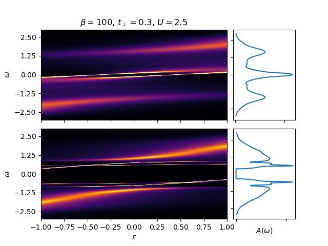
Comparison of the energy resolved spectral functions in the Dimer Hubbard Model in the coexistence region. For the metallic and insulating solution. Figure is discussed in reference [Najera2017]

[Najera2017]

O. Nájera, Civelli, M., V. Dobrosavljevic, & Rozenberg, M. J. (2017). Resolving the VO_2 controversy: Mott mechanism dominates the insulator-to-metal transition. Physical Review B, 95(3), 035113. http://dx.doi.org/10.1103/physrevb.95.035113

# Author: Óscar Nájera

from __future__ import (absolute_import, division, print_function,
                        unicode_literals)

import matplotlib.pyplot as plt
import numpy as np

import dmft.common as gf
import dmft.dimer as dimer
import dmft.ipt_imag as ipt


def ipt_u_tp(u_int, tp, beta, seed='ins'):
    tau, w_n = gf.tau_wn_setup(dict(BETA=beta, N_MATSUBARA=2**12))
    giw_d, giw_o = dimer.gf_met(w_n, 0., 0., 0.5, 0.)
    if seed == 'ins':
        giw_d, giw_o = 1 / (1j * w_n + 4j / w_n), np.zeros_like(w_n) + 0j

    giw_d, giw_o, loops = dimer.ipt_dmft_loop(
        beta, u_int, tp, giw_d, giw_o, tau, w_n, 1e-13)
    g0iw_d, g0iw_o = dimer.self_consistency(
        1j * w_n, 1j * giw_d.imag, giw_o.real, 0., tp, 0.25)
    siw_d, siw_o = ipt.dimer_sigma(u_int, tp, g0iw_d, g0iw_o, tau, w_n)

    return siw_d, siw_o, w_n


def calculate_Aw(sig_d, sig_o, w_n, w_set, w, eps_k, tp):
    ss, sa = dimer.pade_diag(1j * sig_d.imag, sig_o.real, w_n, w_set, w)

    lat_gfs = 1 / np.add.outer(-eps_k, w - tp + 7e-3j - ss)
    lat_gfa = 1 / np.add.outer(-eps_k, w + tp + 7e-3j - sa)
    Aw = -.5 * (lat_gfa + lat_gfs).imag / np.pi

    return Aw, ss, sa


def plot_spectra(u_int, tp, beta, w, w_set, eps_k, axes):
    pdm, pam, pdi, pai = axes
    x, y = np.meshgrid(eps_k, w)
    # metal
    siw_d, siw_o, w_n = ipt_u_tp(u_int, tp, beta, 'met')
    Aw, ss, sa = calculate_Aw(siw_d, siw_o, w_n, w_set, w, eps_k, tp)
    Aw = np.clip(Aw, 0, 1,)
    pdm.pcolormesh(x, y, Aw.T, cmap=plt.get_cmap(r'inferno'))
    gsts = gf.semi_circle_hiltrans(w - tp - (ss.real - 1j * np.abs(ss.imag)))
    gsta = gf.semi_circle_hiltrans(w + tp - (sa.real - 1j * np.abs(sa.imag)))
    gloc = 0.5 * (gsts + gsta)
    pam.plot(-gloc.imag / np.pi, w)

    # insulator
    siw_d, siw_o, w_n = ipt_u_tp(u_int, tp, beta, 'ins')
    Aw, ss, sa = calculate_Aw(siw_d, siw_o, w_n, w_set, w, eps_k, tp)
    Aw = np.clip(Aw, 0, 1,)
    pdi.pcolormesh(x, y, Aw.T, cmap=plt.get_cmap(r'inferno'))
    gsts = gf.semi_circle_hiltrans(w - tp - (ss.real - 1j * np.abs(ss.imag)))
    gsta = gf.semi_circle_hiltrans(w + tp - (sa.real - 1j * np.abs(sa.imag)))
    gloc = 0.5 * (gsts + gsta)
    pai.plot(-gloc.imag / np.pi, w)


def write_labels_e_struct(axes):
    axes[0].set_xticklabels([])
    axes[0].set_yticks(np.linspace(-2.5, 2.5, 5))
    axes[1].set_yticks(np.linspace(-2.5, 2.5, 5))
    axes[1].set_yticklabels([])
    axes[1].set_xticklabels([])
    axes[2].set_yticks(np.linspace(-2.5, 2.5, 5))
    axes[3].set_yticks(np.linspace(-2.5, 2.5, 5))
    axes[3].set_yticklabels([])
    axes[3].set_xticklabels([])
    axes[0].set_ylabel(r'$\omega$')
    axes[2].set_ylabel(r'$\omega$')
    axes[2].set_xlabel(r'$\epsilon$')
    axes[3].set_xlabel(r'$A(\omega)$')


w = np.linspace(-3, 3, 1000)
eps_k = np.linspace(-1., 1., 61)
w_set = np.arange(150)
for U in [2.5]:
    fig, ax = plt.subplots(2, 2, gridspec_kw=dict(
        wspace=0.05, hspace=0.1, width_ratios=[3, 1]))
    axes = ax.flatten()
    plot_spectra(U, .3, 100, w, w_set, eps_k, axes)

    write_labels_e_struct(axes)
    axes[0].set_title(
        r"$\beta={}$, $t_\perp={}$, $U={}$".format(100, .3, U))

#plt.savefig('ipt_arpes_MIT.pdf', format='pdf', transparent=False, bbox_inches='tight', pad_inches=0.05)

Total running time of the script: ( 0 minutes 1.263 seconds)