Scattering rates change in Temperature
Explore the low energy expansion of the Matsubara self-energy. The zero frequency value being the scattering rate. Figure is discussed in reference [Najera2017]
| [Najera2017] | O. Nájera, Civelli, M., V. Dobrosavljevic, & Rozenberg, M. J. (2017). Resolving the VO_2 controversy: Mott mechanism dominates the insulator-to-metal transition. Physical Review B, 95(3), 035113. http://dx.doi.org/10.1103/physrevb.95.035113 |
# Created Mon Mar  7 01:14:02 2016
# Author: Óscar Nájera

from __future__ import division, absolute_import, print_function

from math import log, ceil
import numpy as np
import matplotlib.pyplot as plt
import dmft.dimer as dimer
import dmft.common as gf
import dmft.ipt_imag as ipt


def loop_beta(u_int, tp, betarange, seed='ins'):
    """Solves IPT dimer and return Im Sigma_AA, Re Simga_AB

    returns list len(betarange) x 2 Sigma arrays """

    sigma_iw = []
    iterations = []
    for beta in betarange:
        tau, w_n = gf.tau_wn_setup(
            dict(BETA=beta, N_MATSUBARA=max(2**ceil(log(4 * beta) / log(2)), 256)))
        giw_d, giw_o = dimer.gf_met(w_n, 0., 0., 0.5, 0.)
        if seed == 'ins':
            giw_d, giw_o = 1 / (1j * w_n - 4j / w_n), np.zeros_like(w_n) + 0j

        giw_d, giw_o, loops = dimer.ipt_dmft_loop(
            beta, u_int, tp, giw_d, giw_o, tau, w_n, 1e-3)
        iterations.append(loops)
        g0iw_d, g0iw_o = dimer.self_consistency(
            1j * w_n, 1j * giw_d.imag, giw_o.real, 0., tp, 0.25)
        siw_d, siw_o = ipt.dimer_sigma(u_int, tp, g0iw_d, g0iw_o, tau, w_n)
        sigma_iw.append((siw_d.imag, siw_o.real))

    print(np.array(iterations))

    return sigma_iw
Calculate the dimer solution for Metals up to Uc2 in the in the given temperature range. Include the behavior of 2 insulators inside the coexistence region.
temp = np.arange(1 / 500., .05, .001)
BETARANGE = 1 / temp

U_intm = np.linspace(0, 3, 13)
sigmasM_U = [loop_beta(u_int, .3, BETARANGE, 'met') for u_int in U_intm]

U_inti = [2.5, 3.]
sigmasI_U = [loop_beta(u_int, .3, BETARANGE, 'ins') for u_int in U_inti]
Out:
[487 327 245 198 162 142 126 111 100  90  85  75  70  65  64  59  59  54
  49  49  49  44  44  44  39  39  38  34  34  34  33  33  29  29  29  28
  28  28  28  28  24  24  23  23  23  23  23  23]
[481 322 239 193 162 136 121 106 100  90  80  75  70  64  64  59  54  54
  49  49  44  44  44  39  39  39  38  34  34  33  33  33  29  29  28  28
  28  28  28  24  24  23  23  23  23  23  23  23]
[464 310 233 187 156 131 115 105  95  85  79  74  69  64  59  54  54  49
  49  44  44  43  39  39  38  34  34  33  33  33  29  29  28  28  28  28
  24  24  23  23  23  23  23  23  23  23  19  19]
[435 287 216 175 145 125 109  99  89  79  74  69  64  59  54  49  48  44
  43  43  38  38  38  33  33  33  33  29  28  28  28  28  28  24  23  23
  23  23  23  23  23  19  19  19  19  19  18  18]
[405 269 199 158 133 113  98  88  78  73  68  63  58  53  48  48  43  43
  38  38  38  33  33  33  32  28  28  28  28  24  23  23  23  23  23  23
  19  19  19  19  18  18  18  18  18  18  18  17]
[364 245 180 146 121 101  87  77  72  62  57  52  52  47  42  42  37  37
  33  33  32  28  28  28  27  27  23  23  23  23  23  19  19  18  18  18
  18  18  18  18  17  14  14  14  14  14  14  14]
[331 219 162 128 104  89  79  70  60  56  51  46  42  41  37  36  32  32
  31  27  27  27  23  23  23  22  22  19  18  18  18  18  18  18  17  14
  14  14  14  14  14  14  14  13  13  13  10  10]
[296 193 142 110  91  77  68  58  54  49  45  40  36  35  31  31  27  26
  26  22  22  22  22  18  18  18  18  17  14  14  14  14  14  14  14  13
  13  12  11  10  10  10  10  10  10  10  10   9]
[265 171 127  96  82  69  60  51  47  42  38  34  30  29  25  25  25  21
  21  21  17  17  17  17  16  13  13  13  13  13  12  11  10  10  10  10
   9   9   9  10  10  11  11  12  12  12  12  13]
[236 148 110  85  69  57  48  44  40  36  32  28  24  24  23  20  20  17
  16  16  13  13  13  13  12  10  10   9   9   9  10  11  11  12  12  13
  13  14  14  14  15  15  15  15  16  16  16  16]
[205 128  94  71  56  48  40  36  30  26  25  22  19  18  18  15  15  12
  12  12  11   9  10  11  11  12  12  13  14  14  15  16  16  17  17  18
  18  18  19  19  19  19  20  20  20  20  20  20]
[175 107  73  56  46  36  30  26  23  20  17  16  14  13  12  12  12  12
  12  13  13  14  15  15  16  17  18  19  20  21  22  23  23  24  25  25
  26  26  26  27  27  27  27  27  27  27  26  26]
[138  80  54  42  33  27  22  19  16  14  12  12  13  13  14  15  15  16
  18  19  21  22  24  26  29  31  33  35  37  39  41  42  43  43  44  44
  43  43  42  41  40  39  38  37  36  35  34  33]
[ 9  9  9  9  9  9  9  9  9  9  9  9  9  9  9 10 10 10 10 11 12 13 18 47 28
 23 21 16 15 15 18 16 15 18 12 20 20 19 18 21 20 21 21 21 21 17 17 21]
[ 7  7  7  7  7  7  7  7  7  7  7  7  7  7  7  7  7  7  7  7  7  7  7  7  7
  7  8  8  8  8  9  9 10 11 12 14 17 27 55 39 32 29 27 25 23 22 21 20]
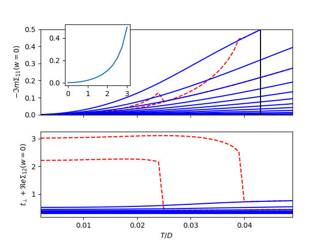
Plot the zero frequency extrapolation of the self-energy. Top panel shows for all metals how upon cooling they become more coherent. Interestingly enough is the insulators is red showning even higher coherence(lower value of the scattering rate) than the metal. This is how the dimer Mott insulator fundamentally differs from the Single Site DMFT Mott insulator. When performing a correct analytical continuation of the Self-energy on the insulator it becomes evident that it is gaped at zero frequency.
The lower panel shows the effective hybridization of the dimers. It is barely changed in the metal but is strongly boosted in the insulator.
def plot_zero_w(function_array, iter_range, tp, betarange, ax, color):
    """Plot the zero frequency extrapolation of a function
    Parameters
    ----------
    function_array: real ndarray
      contains the function (G, Sigma) to linearly fit over 2 first frequencies
    iter_range: list floats
      values of changing variable U or tp
    berarange: real ndarray 1D, values of beta
    entry: 0, 1 corresponds to diagonal or off-diagonal entry of function
    label_head: string for label
    ax, dx: matplotlib axis to plot in
    """

    sig_11_0 = []
    rtp = []
    for j, u in enumerate(iter_range):
        sig_11_0.append([])
        rtp.append([])
        for i, beta in list(enumerate(betarange)):
            tau, w_n = gf.tau_wn_setup(dict(BETA=beta, N_MATSUBARA=2))
            sig_11_0[j].append(np.polyfit(
                w_n, function_array[j][i][0][:2], 1)[1])
            rtp[j].append(np.polyfit(w_n, function_array[j][i][1][:2], 1)[1])

        ax[0].plot(1 / BETARANGE, -np.array(sig_11_0[j]), color, label=str(u))
        ax[1].plot(1 / BETARANGE, tp + np.array(rtp[j]), color, label=str(u))
    ax[0].set_ylabel(r'$-\Im m \Sigma_{11}(w=0)$')
    ax[1].set_ylabel(r'$t_\perp + \Re e\Sigma_{12}(w=0)$')
    ax[1].set_xlabel('$T/D$')
    ax[1].set_xlim([min(temp), max(temp)])

    return np.array(sig_11_0)


fig, si = plt.subplots(2, 1, sharex=True)
sig_11_0i = plot_zero_w(sigmasI_U, U_inti, .3, BETARANGE, si, 'r--')
# fig, si = plt.subplots(2, 1, sharex=True)
sig_11_0m = plot_zero_w(sigmasM_U, U_intm, .3, BETARANGE, si, 'b')
si[0].set_ylim([0, 0.5])

ax = fig.add_axes([.2, .65, .2, .25])
ax.plot(U_intm, -sig_11_0m[:, -7])
ax.set_xticks(np.arange(0, 3.1, 1))
si[0].axvline(temp[-7], color='k')
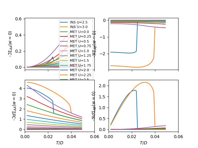
Plot the derivative at zero frequency of the self-energy
def plot_der_zero_w(function_array, iter_range, betarange, entry, label_head, ax, dx):
    """Plot the zero frequency extrapolation of a function
    Parameters
    ----------
    function_array: real ndarray
      contains the function (G, Sigma) to linearly fit over 2 first frequencies
    iter_range: list floats
      values of changing variable U or tp
    berarange: real ndarray 1D, values of beta
    entry: 0, 1 corresponds to diagonal or off-diagonal entry of function
    label_head: string for label
    ax, dx: matplotlib axis to plot in
    """

    for j, u in enumerate(iter_range):
        dat = []
        for i, beta in list(enumerate(betarange)):
            tau, w_n = gf.tau_wn_setup(dict(BETA=beta, N_MATSUBARA=20))
            dat.append(np.polyfit(
                w_n[:2], function_array[j][i][entry][:2], 1))
        ax.plot(1 / BETARANGE, -np.array(dat)
                [:, 1], label=label_head + str(u))
        dx.plot(1 / BETARANGE, -np.array(dat)
                [:, 0], label=label_head + str(u))


f, (si, ds) = plt.subplots(2, 2, sharex=True)
plot_der_zero_w(sigmasI_U, U_inti, BETARANGE, 0, 'INS U=', si[0], ds[0])
plot_der_zero_w(sigmasM_U, U_intm, BETARANGE, 0, 'MET U=', si[0], ds[0])

plot_der_zero_w(sigmasI_U, U_inti, BETARANGE, 1, 'INS U=', si[1], ds[1])
plot_der_zero_w(sigmasM_U, U_intm, BETARANGE, 1, 'MET U=', si[1], ds[1])

si[0].legend(loc=0, prop={'size': 8})

si[0].set_ylabel(r'-$\Im \Sigma_{AA}(w=0)$')
ds[0].set_ylabel(r'-$\Im d\Sigma_{AA}(w=0)$')
si[1].set_ylabel(r'-$\Re \Sigma_{AB}(w=0)$')
ds[1].set_ylabel(r'-$\Re d\Sigma_{AB}(w=0)$')
ds[0].set_xlim([0, .06])

ds[0].set_xlabel('$T/D$')
ds[1].set_xlabel('$T/D$')
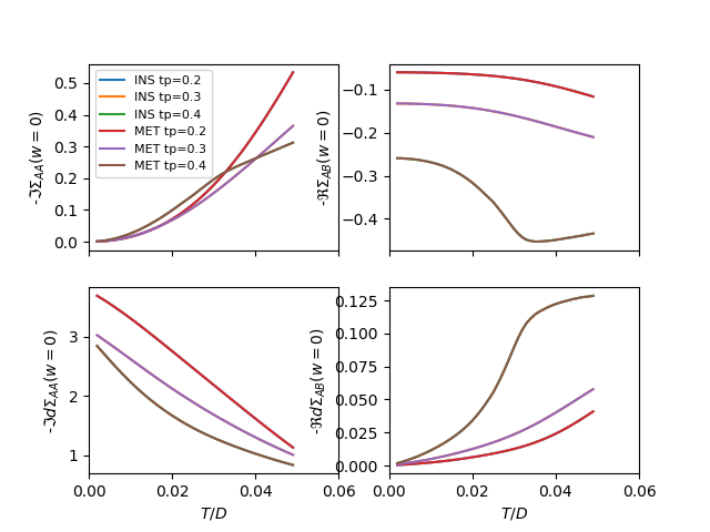
Changing tp in the METAL dome for metal and insulator Fix U
tp_r = [0.2, 0.3, 0.4]
sigmasM_tp = [loop_beta(2.7, tp, BETARANGE, 'M') for tp in tp_r]
sigmasI_tp = [loop_beta(2.7, tp, BETARANGE, 'I') for tp in tp_r]

f, (si, ds) = plt.subplots(2, 2, sharex=True)
plot_der_zero_w(sigmasI_tp, tp_r, BETARANGE, 0, 'INS tp=', si[0], ds[0])
plot_der_zero_w(sigmasM_tp, tp_r, BETARANGE, 0, 'MET tp=', si[0], ds[0])

plot_der_zero_w(sigmasI_tp, tp_r, BETARANGE, 1, 'INS tp=', si[1], ds[1])
plot_der_zero_w(sigmasM_tp, tp_r, BETARANGE, 1, 'MET tp=', si[1], ds[1])

si[0].set_ylabel(r'-$\Im \Sigma_{AA}(w=0)$')
ds[0].set_ylabel(r'-$\Im d\Sigma_{AA}(w=0)$')
si[1].set_ylabel(r'-$\Re \Sigma_{AB}(w=0)$')
ds[1].set_ylabel(r'-$\Re d\Sigma_{AB}(w=0)$')
ds[0].set_xlim([0, .06])

si[0].legend(loc=0, prop={'size': 8})
ds[0].set_xlabel('$T/D$')
ds[1].set_xlabel('$T/D$')
Out:
[129  82  64  46  40  34  29  28  23  18  18  18  14  14  13  12  13  15
  16  17  17  18  18  18  19  19  19  19  19  19  19  19  19  18  18  18
  18  18  18  17  17  17  17  16  16  16  16  16]
[183 110  79  58  47  40  33  27  24  23  20  17  16  14  13  12  12  11
  11  12  12  13  14  14  15  16  17  18  19  19  20  21  22  22  23  23
  24  24  24  25  25  25  25  25  25  25  25  25]
[157  96  64  47  38  30  24  20  17  14  12  10   9   9   9  10  10  10
  10  10  10   9   9   9  13  16  19  22  25  27  28  28  26  25  23  21
  20  19  18  17  16  15  15  14  14  13  12  12]
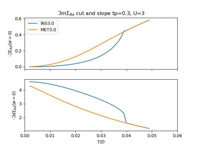
Fine graphics
f, (si, ds) = plt.subplots(2, 1, sharex=True)
plot_der_zero_w([sigmasI_U[1]], [3.], BETARANGE, 0, 'INS', si, ds)
plot_der_zero_w([sigmasM_U[-1]], [3.], BETARANGE, 0, 'MET', si, ds)
si.set_title(r'$\Im m\Sigma_{Aa}$ cut and slope tp=0.3, U=3')
si.set_ylabel(r'-$\Im \Sigma_{AA}(w=0)$')
ds.set_ylabel(r'-$\Im d\Sigma_{AA}(w=0)$')
ds.set_xlim([0, .06])
si.legend(loc=0, prop={'size': 10})
ds.set_xlabel('$T/D$')
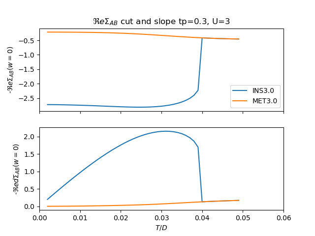
f, (si, ds) = plt.subplots(2, 1, sharex=True)
plot_der_zero_w([sigmasI_U[1]], [3.], BETARANGE, 1, 'INS', si, ds)
plot_der_zero_w([sigmasM_U[-1]], [3.], BETARANGE, 1, 'MET', si, ds)
si.set_title(r'$\Re e\Sigma_{AB}$ cut and slope tp=0.3, U=3')
si.set_ylabel(r'-$\Re e \Sigma_{AB}(w=0)$')
ds.set_ylabel(r'-$\Re e d\Sigma_{AB}(w=0)$')
ds.set_xlim([0, .06])
si.legend(loc=0, prop={'size': 10})
ds.set_xlabel('$T/D$')
Total running time of the script: ( 1 minutes 30.980 seconds)