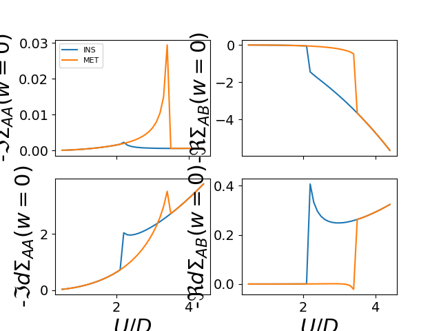
Scattering rates change across the Metal Insulator Transition

Explore the low energy expansion of the Matsubara self-energy. The zero frequency value being the scattering rate.

# Created Mon Mar  7 01:14:02 2016
# Author: Óscar Nájera

from __future__ import division, absolute_import, print_function

from math import log, ceil
import numpy as np
import matplotlib.pyplot as plt
import dmft.dimer as dimer
import dmft.common as gf
import dmft.ipt_imag as ipt
plt.matplotlib.rcParams.update({'axes.labelsize': 22,
                                'xtick.labelsize': 14, 'ytick.labelsize': 14,
                                'axes.titlesize': 22})


def loop_u_tp(u_range, tp_range, beta, seed='mott gap'):
    """Solves IPT dimer and return Im Sigma_AA, Re Simga_AB

    returns list len(betarange) x 2 Sigma arrays
"""
    tau, w_n = gf.tau_wn_setup(
        dict(BETA=beta, N_MATSUBARA=max(2**ceil(log(4 * beta) / log(2)), 256)))
    giw_d, giw_o = dimer.gf_met(w_n, 0., 0., 0.5, 0.)
    if seed == 'I':
        giw_d, giw_o = 1 / (1j * w_n - 4j / w_n), np.zeros_like(w_n) + 0j

    sigma_iw = []
    iterations = []
    for tp, u_int in zip(tp_range, u_range):
        giw_d, giw_o, loops = dimer.ipt_dmft_loop(
            beta, u_int, tp, giw_d, giw_o, tau, w_n, 1e-3)
        iterations.append(loops)
        g0iw_d, g0iw_o = dimer.self_consistency(
            1j * w_n, 1j * giw_d.imag, giw_o.real, 0., tp, 0.25)
        siw_d, siw_o = ipt.dimer_sigma(u_int, tp, g0iw_d, g0iw_o, tau, w_n)
        sigma_iw.append((siw_d.imag, siw_o.real))

    print(np.array(iterations))

    return sigma_iw

U_int = np.arange(.5, 4.5, 0.1)
sigmasM_Ur = loop_u_tp(U_int, .3 * np.ones_like(U_int), 200., 'M')
sigmasI_Ur = loop_u_tp(U_int[::-1], .3 * np.ones_like(U_int), 200., 'I')[::-1]

Out:

[187  17  27  31  22  36  31  31  35  40  44  39  38  42  41  40  39  38
  37  40  35  34  32  30  28  24  22  19  16  13  12   4   4   4   4   4
   4   4   4   3]
[  5   4   4   4   4   4   4   4   4   4   4   4   4   4   5   5   5   6
   6   6   8  10  14 119  41  46  42  43  43  44  40  45  40  41  31  27
  36  22  32  26]

def plot_zero_w(function_array, iter_range, beta, entry, label_head, ax, dx):
    """Plot the zero frequency extrapolation of a function
    Parameters
    ----------
    function_array: real ndarray
      contains the function (G, Sigma) to linearly fit over 2 first frequencies
    iter_range: list floats
      values of changing variable U or tp
    berarange: real ndarray 1D, values of beta
    entry: 0, 1 corresponds to diagonal or off-diagonal entry of function
    label_head: string for label
    ax, dx: matplotlib axis to plot in
    """
    tau, w_n = gf.tau_wn_setup(dict(BETA=beta, N_MATSUBARA=20))

    dat = []
    for j, u in enumerate(iter_range):
        dat.append(np.polyfit(w_n[:2], function_array[j][entry][:2], 1))
    ax.plot(iter_range, -np.array(dat)[:, 1], label=label_head)
    dx.plot(iter_range, -np.array(dat)[:, 0], label=label_head)


f, (si, ds) = plt.subplots(2, 2, sharex=True)
plot_zero_w(sigmasI_Ur, U_int, 100., 0, 'INS', si[0], ds[0])
plot_zero_w(sigmasM_Ur, U_int, 100., 0, 'MET', si[0], ds[0])
plot_zero_w(sigmasI_Ur, U_int, 100., 1, 'INS', si[1], ds[1])
plot_zero_w(sigmasM_Ur, U_int, 100., 1, 'MET', si[1], ds[1])

si[0].legend(loc=0, prop={'size': 8})

si[0].set_ylabel(r'-$\Im \Sigma_{AA}(w=0)$')
ds[0].set_ylabel(r'-$\Im d\Sigma_{AA}(w=0)$')
si[1].set_ylabel(r'-$\Re \Sigma_{AB}(w=0)$')
ds[1].set_ylabel(r'-$\Re d\Sigma_{AB}(w=0)$')

ds[0].set_xlabel('$U/D$')
ds[1].set_xlabel('$U/D$')

Total running time of the script: ( 0 minutes 5.798 seconds)