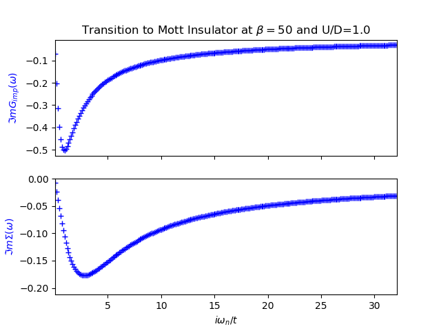
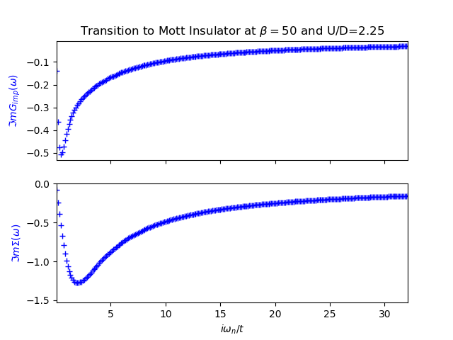
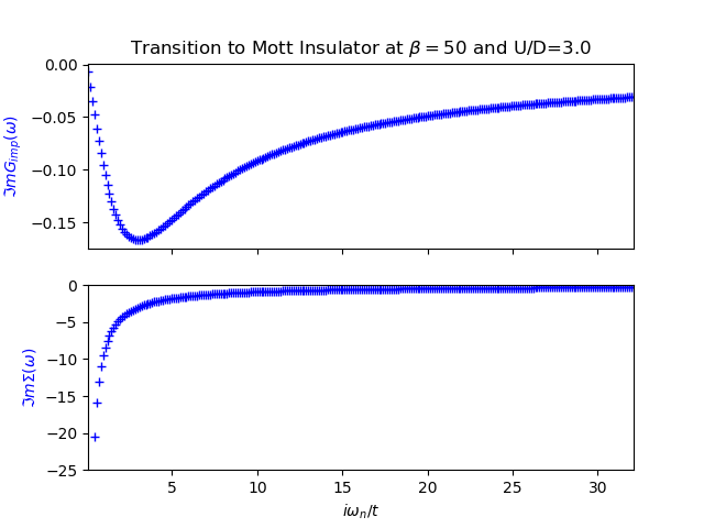
Following the Metal to Mott insulator Transition

Sequence of plots showing the transfer of spectral weight for a Hubbard Model in the Bethe Lattice as the local interaction is raised.

• 
• 
• 
• 

# Code source: Óscar Nájera
# License: BSD 3 clause
from __future__ import division, absolute_import, print_function
import matplotlib.pyplot as plt
import numpy as np
from dmft.twosite import refine_mat_solution

axis = 'matsubara'
du = 0.05
beta = 50
u_int = [2., 4.5, 5.85, 6.]

out_file = axis+'_halffill_b{}_dU{}'.format(beta, du)
res = np.load(out_file+'.npy')

for u in u_int:
    ind = np.abs(res[:, 0] - u).argmin()

    f, (ax1, ax2) = plt.subplots(2, sharex=True)
    ax1.set_title('Transition to Mott Insulator at '
                  '$\\beta=${} and U/D={}'.format(beta, u/2))

    sim = refine_mat_solution(res[ind, 2], u)

    w = sim.omega.imag
    s = sim.GF[r'$\Sigma$']
    g = sim.GF['Imp G']

    ax1.plot(w, g.imag, 'b+')
    ax1.set_xlim([w.min(), w.max()])

    ax2.plot(w, s.imag, 'b+')
    bound = s.imag.min() * 1.2
    ax2.set_ylim([np.max([bound, -25]), 0])

    ax1.set_ylabel(r'$\Im m G_{imp}(\omega)$', color='b')
    ax2.set_ylabel(r'$\Im m \Sigma(\omega)$', color='b')
    ax2.set_xlabel('$i\\omega_n / t$')

Total running time of the script: ( 0 minutes 0.745 seconds)