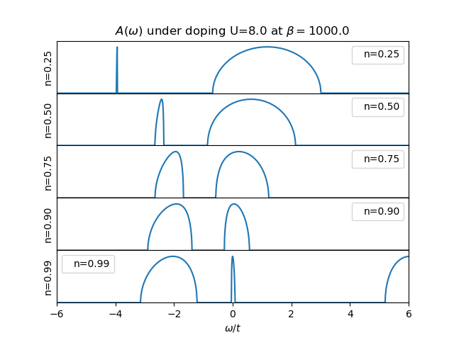
Following the Metal to Mott insulator Transition

Sequence of plots showing the transfer of spectral weight for a Hubbard Model in the Bethe Lattice as the local dopping is increased.

# Code source: Óscar Nájera
# License: BSD 3 clause

from __future__ import division, absolute_import, print_function
import matplotlib.pyplot as plt
import numpy as np
from slaveparticles.quantum import dos

axis = 'real'
u = 8.0
beta = 1e3
dop = [0.25, 0.5, 0.75, 0.9, 0.99]
out_file = axis+'_dop_b{}_U{}'.format(beta, u)
res = np.load(out_file+'.npy')

f, axes = plt.subplots(len(dop), sharex=True)
axes[0].set_title(r'$A(\omega)$ under doping U={} at '
                  '$\\beta=${}'.format(u, beta))
axes[-1].set_xlabel('$\\omega / t$')
f.subplots_adjust(hspace=0)

for ax, n in zip(axes, dop):
    ind = np.abs(res[:, 0] - n).argmin()
    sim = res[ind, 1]

    w = sim.omega
    s = sim.GF[r'$\Sigma$']
    ra = w + sim.mu - s
    rho = dos.bethe_lattice(ra, sim.t)

    ax.plot(w, rho,
            label='n={:.2f}'.format(sim.ocupations().sum()))
    ax.set_xlim([-6, 6])
    ax.set_ylim([0, 0.36])
    ax.set_yticks([])
    ax.set_ylabel('n={:.2f}'.format(sim.ocupations().sum()))
    ax.legend(loc=0, handlelength=0)

Total running time of the script: ( 0 minutes 0.397 seconds)