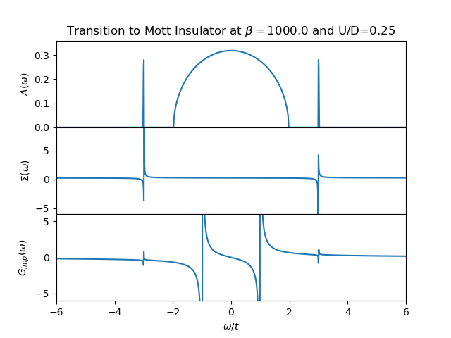
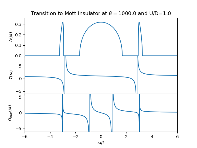
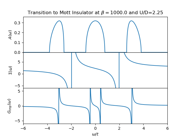
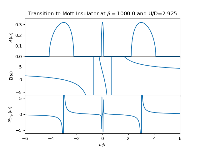
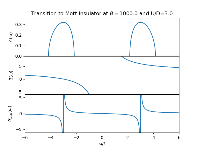
Following the Metal to Mott insulator Transition

Sequence of plots showing the transfer of spectral weight for a Hubbard Model in the Bethe Lattice as the local interaction is raised.

• 
• 
• 
• 
• 

# Code source: Óscar Nájera
# License: BSD 3 clause
from __future__ import division, absolute_import, print_function
import matplotlib.pyplot as plt
import numpy as np
from slaveparticles.quantum import dos

axis = 'real'
du = 0.05
beta = 1e3
u_int = [0.5, 2., 4.5, 5.85, 6.]
out_file = axis+'_halffill_b{}_dU{}'.format(beta, du)
res = np.load(out_file+'.npy')

for u in u_int:
    ind = np.where(np.abs(res[:, 0] - u) < 1e-3)[0][0]

    f, (ax1, ax2, ax3) = plt.subplots(3, sharex=True)
    ax1.set_title('Transition to Mott Insulator at '
                  '$\\beta=${} and U/D={}'.format(beta, u/2))
    f.subplots_adjust(hspace=0)

    w = res[ind, 2].omega
    s = res[ind, 2].GF[r'$\Sigma$']
    g = res[ind, 2].GF['Imp G']
    ra = w+u/2.-s
    rho = dos.bethe_lattice(ra, res[ind, 2].t)

    ax1.plot(w, rho)
    ax1.set_xlim([-6, 6])
    ax1.set_ylim([0, 0.36])

    ax2.plot(w, s)
    ax2.set_ylim([-6, 9])

    ax3.plot(w, g)
    ax3.set_ylim([-6, 6])

    ax1.set_ylabel(r'$A(\omega)$')
    ax2.set_ylabel(r'$\Sigma(\omega)$')
    ax3.set_ylabel(r'$G_{imp}(\omega)$')
    ax3.set_xlabel('$\\omega / t$')

Total running time of the script: ( 0 minutes 1.221 seconds)