Spectral dispersion of insulator

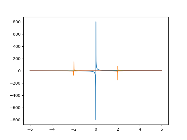
What does the insulator show for Hubbard bands. They are sharp as in the Hubbard I approximation.

• 
• 

Out:

4 9.2695705889e-06 [ 0.5  0.5]

# Author: Óscar Nájera
# License: BSD 3 clause

from __future__ import division, absolute_import, print_function
import matplotlib.pyplot as plt
import numpy as np
from dmft.twosite import TwoSite_Real
from slaveparticles.quantum import dos
import dmft.common as gf

fig = plt.figure()

solver = TwoSite_Real
U = 4
beta = 1e5
sim = solver(beta, 0.5)
sim.mu = U / 2
convergence = False
hyb = 0.4
while not convergence:
    old = hyb
    sim.solve(U / 2, U, old)
    hyb = sim.hyb_V()
    hyb = (hyb + old) / 2
    convergence = np.abs(old - hyb) < 1e-5

print(U, hyb, sim.ocupations())
sim.solve(U / 2, U, hyb)
hyb = sim.hyb_V()

plt.plot(sim.omega, sim.GF[r'$\Sigma$'])
plt.plot(sim.omega, sim.GF[r'Imp G'])

w = sim.omega
s = sim.GF[r'$\Sigma$']
g = sim.GF['Imp G']
ra = w + sim.mu - s
rho = dos.bethe_lattice(ra, sim.t)
plt.plot(w, rho)
g = gf.semi_circle_hiltrans(ra + 0.01j)
plt.plot(w, g.imag)

plt.figure()
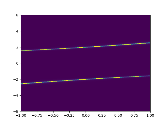
eps_k = np.linspace(-1., 1., 61)
lat_gfs = 1 / np.add.outer(-eps_k, ra + 0.01j)
Aw = np.clip(-lat_gfs.imag / np.pi, 0, 2,)
x, y = np.meshgrid(eps_k, w)
plt.pcolormesh(x, y, Aw.T, cmap=plt.get_cmap(r'viridis'), vmin=0, vmax=2)

Total running time of the script: ( 0 minutes 0.292 seconds)