Stability of the solutions in the coexistence region

As the Energy calculations from IPT source is not reliable enough another methods is also tested to find about the first order line in the transition.

# Author: Óscar Nájera

from __future__ import division, absolute_import, print_function
from math import ceil, log
from functools import partial
import numpy as np
import matplotlib.pylab as plt
from dmft.ipt_imag import dmft_loop
from dmft.common import greenF, tau_wn_setup, fit_gf


def hysteresis(beta, u_range):
    log_g = []
    tau, w_n = tau_wn_setup(
        dict(BETA=beta, N_MATSUBARA=max(2**ceil(log(2 * beta) / log(2)), 256)))
    g_iwn = greenF(w_n)
    for u_int in u_range:
        g_iwn = dmft_loop(u_int, 0.5, g_iwn, w_n, tau, conv=1e-4)[0]
        log_g.append(g_iwn)
    dos = np.array([fit_gf(w_n[:3], gfs[:3].imag)(0.) for gfs in log_g])
    return log_g, dos


def point_stability(g_met, g_ins, U, w_n, tau, c):
    mixture = (1 - c) * g_ins + c * g_met
    g_iwn_end, _ = dmft_loop(U, 0.5, mixture, w_n, tau, conv=1e-4)
    return np.dot(g_iwn_end - mixture, mixture)


def stability(beta, metal_g, insulator_g, urange):
    shift = []
    tau, w_n = tau_wn_setup(
        dict(BETA=beta, N_MATSUBARA=max(2**ceil(log(2 * beta) / log(2)), 256)))
    for g_met, g_ins, U in zip(metal_g, insulator_g, urange):
        stab = partial(point_stability, g_met, g_ins, U, w_n, tau)
        shift.append(0.1 * np.sum([stab(c) for c in np.arange(0, 1, .1)]))

    return np.array(shift)

urange = np.linspace(2.4, 3.6, 41)

TEMP = np.arange(1 / 512., .06, 1 / 256)
shift_log = []
dos_log = []
for BETA in 1 / TEMP:
    metalG, Mdos = hysteresis(BETA, urange)
    insulatorG, Idos = hysteresis(BETA, urange[::-1])
    shift_log.append(stability(BETA, metalG, insulatorG[::-1], urange))
    dos_log.append((Mdos, Idos))

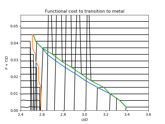
Functional cost for transitioning from insulator to metal

Following Moeller, G., Dobrosavljevi’c, V., & Ruckenstein, A. (1999). RKKY interactions and the Mott transition. Physical Review B, 59(10), 6846–6854. I formulate the expense of transitioning from one solution to the other.

Deltas = np.array(shift_log).real

plt.figure()
for t, df in zip(TEMP, Deltas):
    plt.plot(urange, df + t, 'k')


crossing = [3.39, 3.33, 3.24, 3.12, 3.01,
            2.92, 2.82, 2.73, 2.65, 2.6, 2.54, 2.52]
UC1 = np.array([2.57, 2.57, 2.57, 2.57, 2.55, 2.55,
                2.55, 2.52, 2.52, 2.49, 2.49, 2.49]) + .02
UC2 = np.array([3.39, 3.33, 3.24, 3.18, 3.06, 2.97,
                2.88, 2.78, 2.7, 2.6, 2.54, 2.52])

plt.plot(crossing, TEMP[:len(crossing)], lw=2)
plt.plot(UC1, TEMP[:len(crossing)], lw=2)
plt.plot(UC2, TEMP[:len(crossing)], lw=2)
plt.xlabel(r'$U/D$')
plt.ylabel(r'$F$ + $T/D$')
plt.title('Functional cost to transition to metal')
x, y = np.meshgrid(urange, TEMP)
plt.axis([x.min(), x.max(), 0, y.max()])

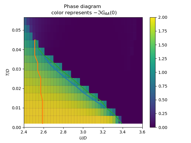
Colorful phase diagram with density of states at Fermi level

metal_dos = np.array(dos_log)[:, 0]
insulator_dos = np.array(dos_log)[:, 1]


plt.figure(1)
plt.pcolormesh(x, y, -metal_dos, cmap=plt.get_cmap(r'viridis'), vmin=0, vmax=2)
plt.colorbar()

z = np.ma.masked_array(-insulator_dos, -insulator_dos > .25)
plt.pcolormesh(x, y, z, alpha=.15, cmap=plt.get_cmap(
    r'viridis'), vmin=0, vmax=2)

plt.axis([x.min(), x.max(), 0, y.max()])
plt.xlabel(r'$U/D$')
plt.ylabel(r'$T/D$')
plt.title(
    'Phase diagram \n color represents $-\\Im G_{{AA}}(0)$')
plt.plot(crossing, TEMP[:len(crossing)], lw=2)
plt.plot(UC1, TEMP[:len(crossing)], lw=2)
plt.plot(UC2, TEMP[:len(crossing)], lw=2)

Total running time of the script: ( 1 minutes 3.563 seconds)