IPT Transition at crossover

Study the end of the crossover region

from __future__ import division, absolute_import, print_function

from dmft.ipt_imag import dmft_loop
from dmft.common import greenF, tau_wn_setup, fit_gf
from dmft.twosite import matsubara_Z

import numpy as np
import matplotlib.pylab as plt


def hysteresis(beta, u_range):
    log_g_sig = []
    tau, w_n = tau_wn_setup(dict(BETA=beta, N_MATSUBARA=beta))
    g_iwn = greenF(w_n)
    for u_int in u_range:
        g_iwn, sigma = dmft_loop(u_int, 0.5, g_iwn, w_n, tau)
        log_g_sig.append((g_iwn, sigma))
    return log_g_sig


U = np.linspace(2.2, 2.5, 100)
results = []
betarange = [16, 17.85, 19.2, 20., 21.3]
for beta in betarange:
    results.append(hysteresis(beta, U))

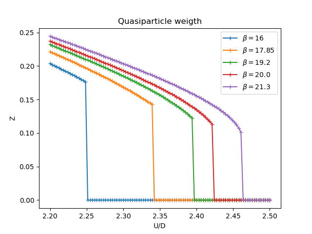
Quasiparticle weight

figz, axz = plt.subplots()
for beta, result in zip(betarange, results):
    u_zet = [matsubara_Z(sigma.imag, beta) for _, sigma in result]
    axz.plot(U, u_zet, '+-', label='$\\beta={}$'.format(beta))
axz.set_title('Quasiparticle weigth')
axz.legend(loc=0)
axz.set_ylabel('Z')
axz.set_xlabel('U/D')

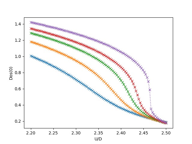
Spectral density at Fermi level

figf, axf = plt.subplots()
for beta, result in zip(betarange, results):
    tau, w_n = tau_wn_setup(dict(BETA=beta, N_MATSUBARA=3))
    u_fl = [-fit_gf(w_n, g_iwn.imag)(0.)for g_iwn, _ in result]
    axf.plot(U, u_fl, 'x:', label='$\\beta={}$'.format(beta))

axf.set_ylabel('Dos(0)')
axz.set_title('Density of states at Fermi level')
axf.set_xlabel('U/D')

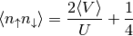
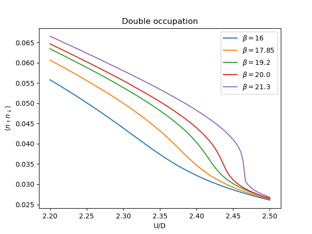
Double occupation

Is proportional to the Potential energy which is defined in Potential energy the tail of this function behaves as

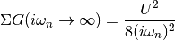
Then to find out the double occupation one uses the relation

figd, axd = plt.subplots()
for beta, result in zip(betarange, results):
    tau, w_n = tau_wn_setup(dict(BETA=beta, N_MATSUBARA=beta))
    V = np.asarray([2 * (0.5 * s * g + u**2 / 8. / w_n**2).real.sum() / beta
                    for (g, s), u in zip(result, U)]) - 0.25 * beta * U**2 / 8.

    D = 2. / U * V + 0.25
    axd.plot(U, D, '-', label='$\\beta={}$'.format(beta))

axd.set_title('Double occupation')
axd.legend(loc=0)
axd.set_ylabel(r'$\langle n_\uparrow n_\downarrow \rangle$')
axd.set_xlabel('U/D')

Total running time of the script: ( 0 minutes 1.452 seconds)