IPT bandwidth controlled

Have a look at the coexistence region and the metal insulator transition from the point of view of a change in bandwidth

from __future__ import division, absolute_import, print_function

from dmft.ipt_imag import dmft_loop
from dmft.common import greenF, tau_wn_setup, fit_gf
from dmft.twosite import matsubara_Z

import numpy as np
import matplotlib.pylab as plt


def hysteresis(beta, D_range):
    log_g_sig = []
    tau, w_n = tau_wn_setup(dict(BETA=beta, N_MATSUBARA=2**11))
    g_iwn = greenF(w_n, D=1)
    for D in D_range:
        g_iwn, sigma = dmft_loop(1, D / 2, g_iwn, w_n, tau)
        log_g_sig.append((g_iwn, sigma))
    return log_g_sig


results = []
Drange = np.linspace(0.25, .75, 61)
Drange = np.concatenate((Drange[::-1], Drange + .005))
betarange = [16, 17.85, 19.2, 20., 21.3, 25, 50, 100, 200, 512]
for beta in betarange:
    results.append(hysteresis(beta, Drange))

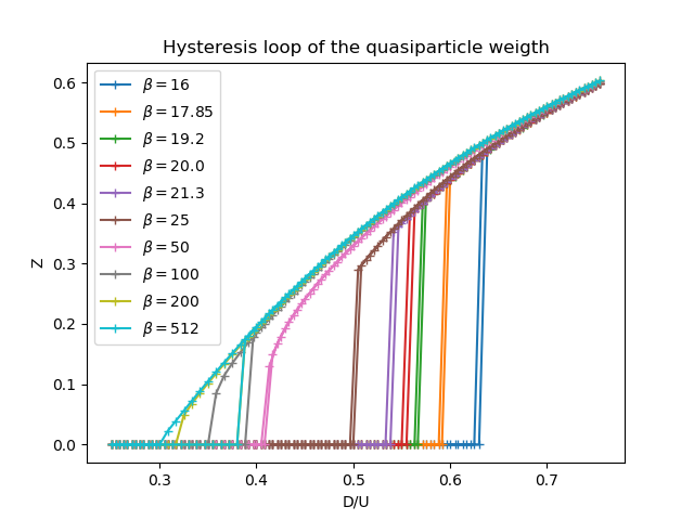
Quasiparticle weight

figz, axz = plt.subplots()
for beta, result in zip(betarange, results):
    u_zet = [matsubara_Z(sigma.imag, beta) for _, sigma in result]
    axz.plot(Drange, u_zet, '+-', label='$\\beta={}$'.format(beta))
    axz.set_title('Hysteresis loop of the quasiparticle weigth')
    axz.legend(loc=0)
    axz.set_ylabel('Z')
    axz.set_xlabel('D/U')

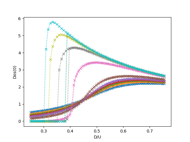
Spectral density at Fermi level

figf, axf = plt.subplots()
for beta, result in zip(betarange, results):
    tau, w_n = tau_wn_setup(dict(BETA=beta, N_MATSUBARA=3))
    u_fl = [-fit_gf(w_n, g_iwn.imag)(0.)for g_iwn, _ in result]
    axf.plot(Drange, u_fl, 'x:', label='$\\beta={}$'.format(beta))

axf.set_ylabel('Dos(0)')
axf.set_xlabel('D/U')

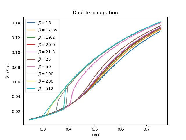
Double occupation

figd, axd = plt.subplots()
for beta, result in zip(betarange, results):
    tau, w_n = tau_wn_setup(dict(BETA=beta, N_MATSUBARA=2**11))
    V = np.asarray([2 * (0.5 * s * g + 1 / 8. / w_n**2).real.sum() / beta
                    for (g, s) in result]) - 0.25 * beta * 1 / 8.

    D = 2. * V + 0.25
    axd.plot(Drange, D, '-', label='$\\beta={}$'.format(beta))

axd.set_title('Double occupation')
axd.legend(loc=0)
axd.set_ylabel(r'$\langle n_\uparrow n_\downarrow \rangle$')
axd.set_xlabel('D/U')

Total running time of the script: ( 0 minutes 31.853 seconds)