Evolution of DOS as function of temperature
Out:
U:  2.5 tp:  0.3
mott gap beta: 500.0  loops:  23
mott gap beta: 250.0  loops:  23
mott gap beta: 166.666666667  loops:  23
mott gap beta: 125.0  loops:  23
mott gap beta: 100.0  loops:  23
mott gap beta: 83.3333333333  loops:  23
mott gap beta: 71.4285714286  loops:  24
mott gap beta: 62.5  loops:  23
mott gap beta: 55.5555555556  loops:  23
mott gap beta: 50.0  loops:  23
mott gap beta: 45.4545454545  loops:  28
mott gap beta: 41.6666666667  loops:  51
mott gap beta: 38.4615384615  loops:  43
mott gap beta: 35.7142857143  loops:  40
mott gap beta: 33.3333333333  loops:  36
mott gap beta: 31.25  loops:  42
mott gap beta: 29.4117647059  loops:  41
mott gap beta: 27.7777777778  loops:  35
mott gap beta: 26.3157894737  loops:  48
mott gap beta: 25.0  loops:  48
U:  2.5 tp:  0.3
met beta: 500.0  loops:  552
met beta: 250.0  loops:  252
met beta: 166.666666667  loops:  158
met beta: 125.0  loops:  111
met beta: 100.0  loops:  85
met beta: 83.3333333333  loops:  66
met beta: 71.4285714286  loops:  54
met beta: 62.5  loops:  45
met beta: 55.5555555556  loops:  38
met beta: 50.0  loops:  31
met beta: 45.4545454545  loops:  28
met beta: 41.6666666667  loops:  25
met beta: 38.4615384615  loops:  27
met beta: 35.7142857143  loops:  31
met beta: 33.3333333333  loops:  35
met beta: 31.25  loops:  39
met beta: 29.4117647059  loops:  42
met beta: 27.7777777778  loops:  44
met beta: 26.3157894737  loops:  47
met beta: 25.0  loops:  48
# Created Tue Jun 14 15:44:38 2016
# Author: Óscar Nájera
from __future__ import division, absolute_import, print_function
import matplotlib.pyplot as plt
plt.matplotlib.rcParams.update({'axes.labelsize': 22,
'xtick.labelsize': 14, 'ytick.labelsize': 14,
'axes.titlesize': 22})
import numpy as np
import dmft.common as gf
import dmft.dimer as dimer
import dmft.ipt_imag as ipt
def loop_beta(u_int, tp, betarange, seed='mott gap'):
"""Solves IPT dimer and return Im Sigma_AA, Re Simga_AB
returns list len(betarange) x 2 Sigma arrays
"""
sigma_iw = []
g_iw = []
lw_n = []
print('U: ', u_int, 'tp: ', tp)
for beta in betarange:
tau, w_n = gf.tau_wn_setup(dict(BETA=beta, N_MATSUBARA=2**12))
lw_n.append(w_n)
giw_d, giw_o = dimer.gf_met(w_n, 0., 0., 0.5, 0.)
if seed == 'mott gap':
giw_d, giw_o = 1 / (1j * w_n - 4j / w_n), np.zeros_like(w_n) + 0j
giw_d, giw_o, loops = dimer.ipt_dmft_loop(
beta, u_int, tp, giw_d, giw_o, tau, w_n, 1e-13)
g_iw.append((giw_d.imag, giw_o.real))
g0iw_d, g0iw_o = dimer.self_consistency(
1j * w_n, 1j * giw_d.imag, giw_o.real, 0., tp, 0.25)
siw_d, siw_o = ipt.dimer_sigma(u_int, tp, g0iw_d, g0iw_o, tau, w_n)
sigma_iw.append((siw_d.imag, siw_o.real))
print(seed, 'beta:', beta, ' loops: ', loops)
return np.array(g_iw), np.array(sigma_iw), np.array(lw_n)
def lin_approx(w_n, rf_iwn):
"""Return the linear approximation at low frequency for green function
w_n: real matsubara frequency
rf_iwn: real valued function of green function
return: float tuple (m, c) corresponding y = m*x+c
"""
dy = rf_iwn[1] - rf_iwn[0]
dx = 2 * w_n[0]
m = dy / dx
c = 3 / 2 * rf_iwn[0] - rf_iwn[1] / 2
return m, c
U = 2.5
tp = 0.3
temp = np.linspace(0.002, 0.04, 20)
betarange = 1 / temp
gi_iw, sigmai_iw, lw_n = loop_beta(U, tp, betarange)
gm_iw, sigmam_iw, lw_n = loop_beta(U, tp, betarange, 'met')
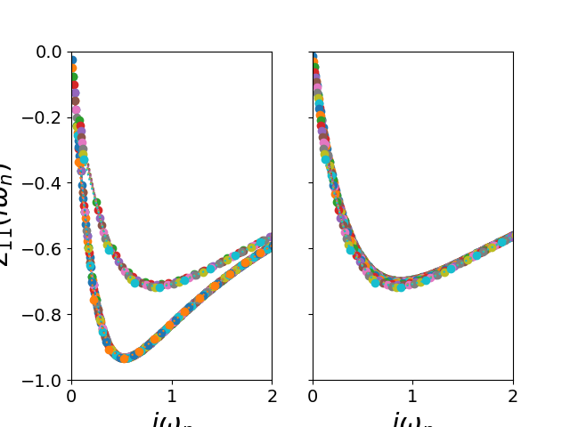
fig, ax_sig = plt.subplots(1, 2, sharex=True, sharey=True)
for (sig_d, sig_o), wn in zip(sigmai_iw, lw_n):
ax_sig[0].plot(wn, sig_d, 'o:')
for (sig_d, sig_o), wn in zip(sigmam_iw, lw_n):
ax_sig[1].plot(wn, sig_d, 'o:')
ax_sig[1].set_xlim([0, 2])
ax_sig[1].set_ylim([-1, 0])
ax_sig[0].set_xlabel(r'$i\omega_n$')
ax_sig[1].set_xlabel(r'$i\omega_n$')
ax_sig[0].set_ylabel(r'$\Sigma_{11}(i\omega_n)$')
# Low freq review G
ins_mc = -np.array([lin_approx(wn, sig_d)
for (sig_d, sig_o), wn in zip(gi_iw, lw_n)]).T
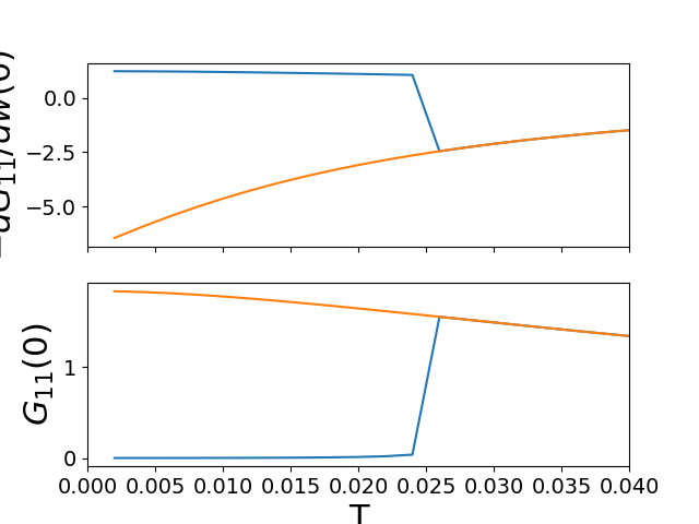
fih, ax_zw = plt.subplots(2, 1, sharex=True)
ax_zw[0].plot(temp, ins_mc[0])
ax_zw[1].plot(temp, ins_mc[1])
met_mc = -np.array([lin_approx(wn, sig_d)
for (sig_d, sig_o), wn in zip(gm_iw, lw_n)]).T
ax_zw[0].plot(temp, met_mc[0])
ax_zw[1].plot(temp, met_mc[1])
ax_zw[1].set_xlabel('T')
ax_zw[0].set_ylabel(r'$-dG_{11}/dw(0)$')
ax_zw[1].set_ylabel(r'$G_{11}(0)$')
ax_zw[1].set_xlim([0, 0.04])
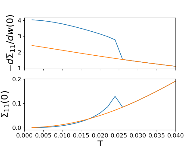
# Low freq review sigma
ins_mc = -np.array([lin_approx(wn, sig_d)
for (sig_d, sig_o), wn in zip(sigmai_iw, lw_n)]).T
fih, ax_zw = plt.subplots(2, 1, sharex=True)
ax_zw[0].plot(temp, ins_mc[0])
ax_zw[1].plot(temp, ins_mc[1])
met_mc = -np.array([lin_approx(wn, sig_d)
for (sig_d, sig_o), wn in zip(sigmam_iw, lw_n)]).T
ax_zw[0].plot(temp, met_mc[0])
ax_zw[1].plot(temp, met_mc[1])
ax_zw[1].set_xlabel('T')
ax_zw[0].set_ylabel(r'$-d\Sigma_{11}/dw(0)$')
ax_zw[1].set_ylabel(r'$\Sigma_{11}(0)$')
ax_zw[1].set_xlim([0, 0.04])
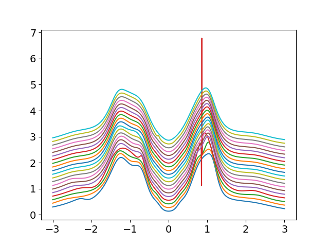
# Pade Continuations
plt.figure()
w = np.linspace(-3, 3, 800)
for (siw_d, siw_o), wn, beta in zip(sigmam_iw, lw_n, betarange):
w_set = 0
if 2 * beta < 150:
w_set = np.arange(150).astype(int)
else:
w_set = np.arange(0, 2 * beta, 2 * beta / 150).astype(int)
sig_ss, sig_sa = dimer.pade_diag(1j * siw_d, siw_o, wn, w_set, w)
plt.plot(w, 70 / beta + np.abs(sig_ss.imag))
for (siw_d, siw_o), wn, beta in list(zip(sigmai_iw, lw_n, betarange)):
w_set = 0
if 2 * beta < 150:
w_set = np.arange(150).astype(int)
else:
w_set = np.arange(0, 2 * beta, 2 * beta / 150).astype(int)
sig_ss, sig_sa = dimer.pade_diag(1j * siw_d, siw_o, wn, w_set, w)
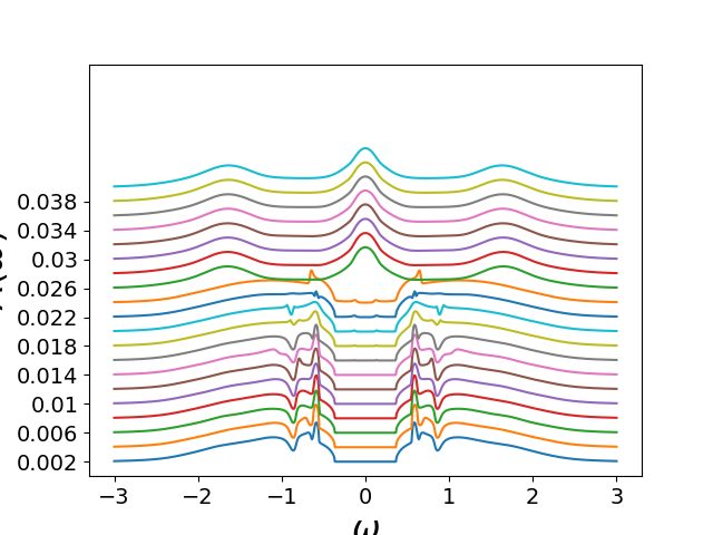
plt.figure('si')
plt.plot(w, 100 / beta + np.abs(sig_ss.imag))
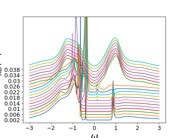
plt.figure('a')
gss_w = gf.semi_circle_hiltrans(
w - tp - (sig_ss.real - 1j * np.abs(sig_ss.imag)))
gsa_w = gf.semi_circle_hiltrans(
w + tp - (sig_sa.real - 1j * np.abs(sig_sa.imag)))
gss_w = .5 * (gss_w + gsa_w)
plt.plot(w, 100 / beta - gss_w.imag / np.pi)
plt.figure('a')
plt.ylim([0, 5.7])
plt.xlabel(r'$\omega$')
plt.ylabel(r'$A(\omega)$')
plt.yticks(100 / betarange[::2], np.around(1 / betarange, 3)[::2])
plt.figure('si')
plt.yticks(100 / betarange[::2], np.around(1 / betarange, 3)[::2])
plt.ylim([0, 7.6])
plt.ylabel(r'$\Im \Sigma_{AB}(\omega)$')
plt.xlabel(r'$\omega$')
Total running time of the script: ( 0 minutes 20.693 seconds)