Landau Theory of the Mott transition
Perform a fit of the order parameter, linked to double occupation to match a Landau theory formulation in correspondence to Kotliar, G., Lange, E., & Rozenberg, M. J. (2000). Landau Theory of the Finite Temperature Mott Transition. Phys. Rev. Lett., 84(22), 5180–5183. http://dx.doi.org/10.1103/PhysRevLett.84.5180
Study above the critical point
Out:
[ 80  87  93  98 103 107 110 112 114 115 116 117 117 117 116 116 115 114
 113 112 111 109 108 106 104 102 100  98  96 104 113 124 138 160 196 281
 363 168 133 116 105  97  91  85  81]
[ 69  75  82  88  93  98 103 107 111 115 118 122 125 127 130 132 134 136
 138 139 140 141 142 143 143 143 143 143 142 141 139 137 135 150 199 469
 133  96  80  71  65  61  57  54  52]
[ 64  70  76  81  86  91  96 100 104 108 112 115 119 122 125 128 131 134
 136 139 141 143 145 147 149 150 152 153 153 154 154 154 153 151 170 283
 149  94  77  67  61  56  53  50  47]
[ 19  20  22  23  25  26  28  29  30  32  33  35  36  38  39  41  42  44
  46  48  50  52  55  57  60  63  67  71  76  82  90  99 112 131 165 253
 270 164 137 122 112 105  99  94  90]
[ 17  18  19  20  22  23  24  25  26  27  28  30  31  32  33  34  36  37
  39  40  42  44  46  48  51  53  57  60  65  70  77  86  99 121 172 261
 107  87  88  72  78  59  71  62  66]
[ 16  17  18  20  21  22  23  24  25  26  27  28  29  30  31  32  33  34
  36  37  39  40  42  44  46  48  51  54  57  61  66  73  82  95 117 175
 182 108  92  84  72  65  64  69  67]
[  4.97099285e+04  -1.67641855e+01  -1.14450295e-01   4.60473231e-02]
[  6.16488749e+04  -1.65614028e+01  -1.02823015e-01   4.88102948e-02]
[  6.11088790e+04  -1.68390446e+01  -1.04283494e-01   4.99004705e-02]
[ -2.13277586e+05   5.99344268e+00   0.00000000e+00   3.37508693e-02]
[ -1.63656897e+05   7.25248650e+00   0.00000000e+00   3.76399507e-02]
[ -1.37368496e+05   8.13142805e+00   0.00000000e+00   3.98125830e-02]
from scipy.optimize import curve_fit
import numpy as np
import matplotlib.pyplot as plt
import dmft.dimer as dimer
import dmft.common as gf
import dmft.ipt_imag as ipt
plt.matplotlib.rcParams.update({'figure.figsize': (8, 8), 'axes.labelsize': 22,
'axes.titlesize': 22, 'figure.autolayout': True})
def dmft_solve(giw_d, giw_o, u_int, tp, beta, tau, w_n):
giw_d, giw_o, loops = dimer.ipt_dmft_loop(
beta, u_int, tp, giw_d, giw_o, tau, w_n)
g0iw_d, g0iw_o = dimer.self_consistency(
1j * w_n, 1j * giw_d.imag, giw_o.real, 0., tp, 0.25)
siw_d, siw_o = ipt.dimer_sigma(u_int, tp, g0iw_d, g0iw_o, tau, w_n)
ekin = dimer.ekin(giw_d, giw_o, w_n, tp, beta)
# last division because I want per spin epot
epot = dimer.epot(giw_d, w_n, beta, u_int ** 2 /
4 + tp**2, ekin, u_int) / 4
return (giw_d, giw_o), (siw_d, siw_o), ekin, epot, loops
def loop_u_tp(u_range, tprange, beta, seed='mott gap'):
tau, w_n = gf.tau_wn_setup(dict(BETA=beta, N_MATSUBARA=256))
giw_d, giw_o = dimer.gf_met(w_n, 0., 0., 0.5, 0.)
if seed == 'ins':
giw_d, giw_o = 1 / (1j * w_n + 4j / w_n), np.zeros_like(w_n) + 0j
sols = [dmft_solve(giw_d, giw_o, u_int, tp, beta, tau, w_n)
for u_int, tp in zip(u_range, tprange)]
giw_s = np.array([g[0] for g in sols])
sigma_iw = np.array([g[1] for g in sols])
ekin = np.array([g[2] for g in sols])
epot = np.array([g[3] for g in sols])
iterations = np.array([g[4] for g in sols])
print(iterations)
return giw_s, sigma_iw, ekin, epot, w_n
# below the critical point
fac = np.arctan(.55 * np.sqrt(3) / .25)
udelta = np.tan(np.linspace(-fac, fac, 71)) * .15 / np.sqrt(3)
udelta = udelta[:int(len(udelta) / 2) + 10]
dudelta = np.diff(udelta)
databm = []
databi = []
bet_ucm = [(24, 3.064),
(28, 3.028),
(30, 3.023),
]
for beta, uc in bet_ucm:
urange = udelta + uc + .07
giw_s, sigma_iw, ekin, epot, w_n = loop_u_tp(
urange, .3 * np.ones_like(urange), beta, 'met')
databm.append(2 * epot / urange - 0.003)
bet_uci = [(24, 3.01),
(28, 2.8),
(30, 2.719),
]
databi = []
for beta, uc in bet_uci:
urange = -udelta + uc + .07
giw_s, sigma_iw, ekin, epot, w_n = loop_u_tp(
urange, .3 * np.ones_like(urange), beta, 'ins')
databi.append(2 * epot / urange - 0.003)
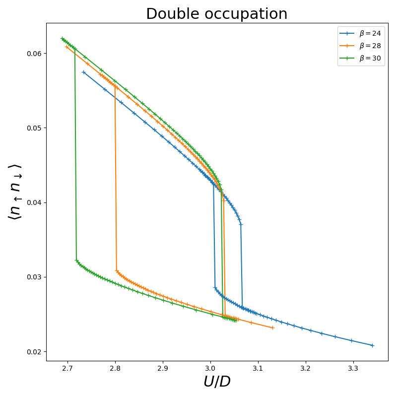
plt.figure()
for dd, (beta, uc) in zip(databm, bet_ucm):
plt.plot(uc + udelta, dd, '+-', label=r'$\beta={}$'.format(beta))
plt.gca().set_color_cycle(None)
d_c = [dc[int(len(udelta) / 2)] for dc in databi]
for dd, dc, (beta, uc) in zip(databi, d_c, bet_uci):
plt.plot(uc - udelta, dd, '+-') # , label=r'$\beta={}$'.format(beta))
plt.title(r'Double occupation')
plt.ylabel(r'$\langle n_\uparrow n_\downarrow \rangle$')
plt.xlabel(r'$U/D$')
plt.legend()
plt.savefig("dimer_tp0.3_docc_bTc.pdf",
transparent=False, bbox_inches='tight', pad_inches=0.05)
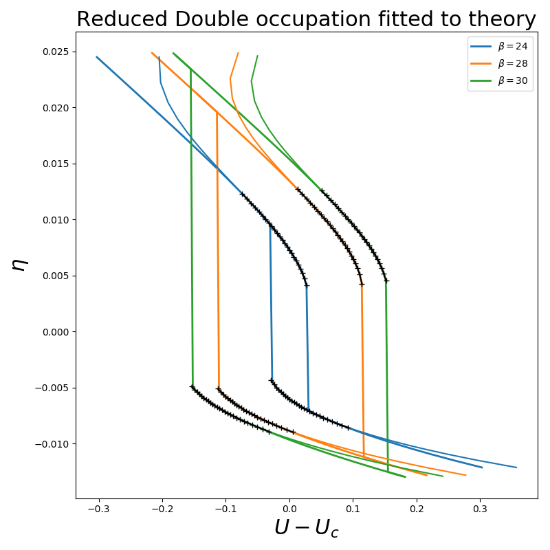
def fit_cube_lin(eta, c, p, q, d):
return (c * (eta - d)**3 + p * (eta - d) + q) # / (1 + q * eta)
u_cen = [0.027, 0.114, 0.152]
plt.figure()
plt.gca().set_color_cycle(None)
bc = [b for b, _ in bet_ucm]
for ddm, ddi, uc, beta in zip(databm, databi, u_cen, bc):
cent = (ddm[-11] + ddi[-11]) / 2
plt.plot(udelta + uc, ddm - cent, '-', lw=2,
label=r'$\beta={}$'.format(beta))
plt.gca().set_color_cycle(None)
for ddm, ddi, uc in zip(databm, databi, u_cen):
cent = (ddm[-11] + ddi[-11]) / 2
plt.plot(-uc - udelta, ddi - cent, '-', lw=2)
plt.gca().set_color_cycle(None)
bb = [9, 9, 9]
lb = 12
bc = [b for b, _ in bet_uci]
for dd, ddi, bound, beta, uc in zip(databm, databi, bb, bc, u_cen):
cent = (dd[-11] + ddi[-11]) / 2
popt, pcov = curve_fit(
fit_cube_lin, dd[lb:-bound], udelta[lb:-bound], p0=[4e4, -17, -.1, 0.035])
ft = fit_cube_lin(dd, *popt) + uc
plt.plot(ft[:-bound], dd[:-bound] - cent)
#plt.plot(ft[lb:-bound], dd[lb:-bound], "k+")
plt.plot(ft[lb:-bound], dd[lb:-bound] - cent, "k+-")
print(popt)
def fit_cube_lin(eta, c, p, q, d):
return (c * (eta - d)**3 + p * (eta - d)) # / (1 + q * eta)
plt.gca().set_color_cycle(None)
bb = [9, 10, 9]
lb = 10
for ddm, dd, bound, uc in zip(databm, databi, bb, u_cen):
cent = (ddm[-11] + dd[-11]) / 2
popt, pcov = curve_fit(
fit_cube_lin, dd[lb:-bound], -udelta[lb:-bound], p0=[-4e4, 7, 0, 0.035])
ft = fit_cube_lin(dd, *popt) - uc
plt.plot(ft[:-bound], dd[:-bound] - cent)
plt.plot(ft[lb:-bound], dd[lb:-bound] - cent, "k+-")
print(popt)
plt.title(r'Reduced Double occupation fitted to theory')
plt.ylabel(r'$\eta$')
plt.xlabel(r'$U-U_c$')
plt.legend()
plt.savefig("dimer_tp0.3_eta_landau_bTc.pdf",
transparent=False, bbox_inches='tight', pad_inches=0.05)
Total running time of the script: ( 0 minutes 33.491 seconds)