The Analytical Structure of a the Green’s Function

Here I plot the form of the Green’s function in the upper complex plane. To show the connection between the Matsubara Green’s function an the real frequency retarded Green’s function.

# Created Sat Aug 13 23:55:28 2016
# Author: Óscar Nájera

from __future__ import division, absolute_import, print_function

import matplotlib.pyplot as plt
import numpy as np
from mpl_toolkits.mplot3d import Axes3D
from dmft.ipt_imag import dmft_loop
from dmft.common import greenF, tau_wn_setup, pade_coefficients, pade_rec, semi_circle_hiltrans

plt.matplotlib.rcParams.update({'axes.labelsize': 22,
                                'axes.titlesize': 22, 'figure.autolayout': True})


def plot_complex_gf(omega, jomega, w_n, function, eps=1e-3):
    O, W = np.meshgrid(omega, np.concatenate(([eps], jomega)))
    Z = O + 1j * W

    green_func = function(Z)
    real_green_func = function(omega + 1j * eps)
    imag_green_func = function(1j * jomega)
    mats_green_func = function(1j * w_n)

    fig = plt.figure()
    ax = fig.gca(projection='3d')

    surf = ax.plot_surface(O, W, green_func.real, color='blue',
                           alpha=0.2, rstride=1, cstride=1, linewidth=0)
    surf = ax.plot_surface(O, W, green_func.imag,
                           color='red', alpha=0.3, rstride=1, cstride=1, linewidth=0)
    ax.plot(omega, np.zeros_like(omega), real_green_func.real, 'b-', lw=3)
    ax.plot(omega, np.zeros_like(omega), real_green_func.imag, 'r-', lw=3)

    ax.plot(np.zeros_like(w_n), w_n, mats_green_func.real, 'bs:')
    ax.plot(np.zeros_like(w_n), w_n, mats_green_func.imag, 'rs:')

    ax.set_xlabel(r'$\omega$')
    ax.set_ylabel(r'$i\omega_n$')
    ax.set_zlabel(r'$G(z)$')
    return ax

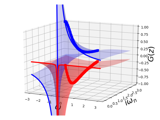
A free single particle

omega = np.linspace(-3, 3, 150)
jomega = np.linspace(1e-4, 3, 100)
ax = plot_complex_gf(omega, jomega, jomega, lambda z: 1 / (z + 0.7))
ax.view_init(15, -64)
ax.set_zlim3d(-1., 1.)

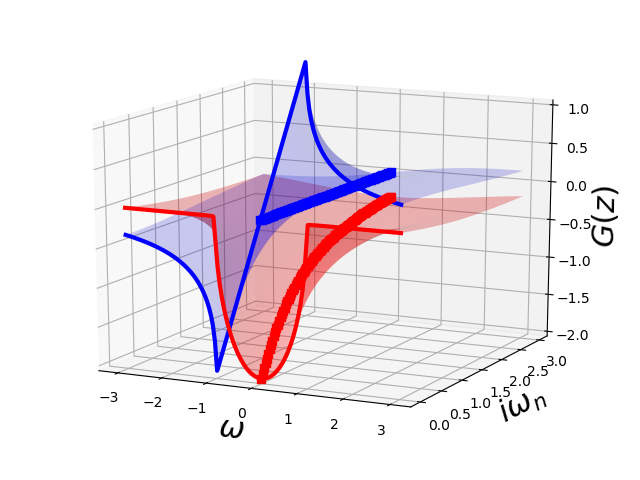
The Semi-Circular Density of states

ax = plot_complex_gf(omega, jomega, jomega, semi_circle_hiltrans)
ax.view_init(15, -64)
ax.set_zlim3d(-2., 1.)

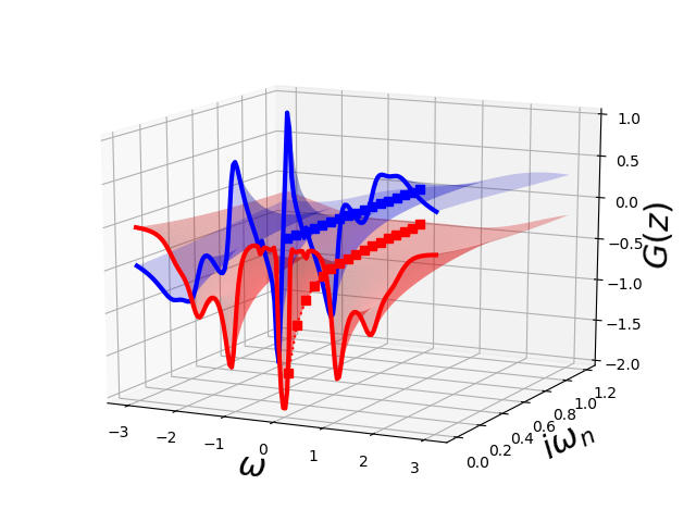
Results from IPT

Starting from the Metallic seed on the Bethe Lattice the DMFT equations are solved iteratively in by perturbation theory in the Matsubara axis. The resulting Green’s function is then approximated by its Padé approximant which allows to evaluate it on the upper complex plane.

beta = 90.
U = 2.7
tau, w_n = tau_wn_setup(dict(BETA=beta, N_MATSUBARA=1024))
g_iwn0 = greenF(w_n)
g_iwn, s_iwn = dmft_loop(U, 0.5, g_iwn0, w_n, tau, conv=1e-12)
x = int(2 * beta)
w_set = np.arange(x)

pc = pade_coefficients(g_iwn[w_set], w_n[w_set])

ax = plot_complex_gf(omega, np.linspace(1e-3, 1.2, 30), w_n[:17],
                     lambda z: pade_rec(pc, z, w_n[w_set]))
ax.view_init(15, -64)
ax.set_zlim3d([-2, 1])

For the insulating solution

U = 3.2
tau, w_n = tau_wn_setup(dict(BETA=beta, N_MATSUBARA=1024))
g_iwn0 = greenF(w_n)
g_iwn, s_iwn = dmft_loop(
    U, 0.5, 1 / (1j * w_n - 1 / g_iwn0), w_n, tau, conv=1e-12)
x = int(2 * beta)
w_set = np.arange(x)

pc = pade_coefficients(g_iwn[w_set], w_n[w_set])

ax = plot_complex_gf(omega, np.linspace(1e-3, 1.2, 30), w_n[:17],
                     lambda z: pade_rec(pc, z, w_n[w_set]))
ax.view_init(15, -60)
ax.set_zlim3d([-1.3, 0.7])

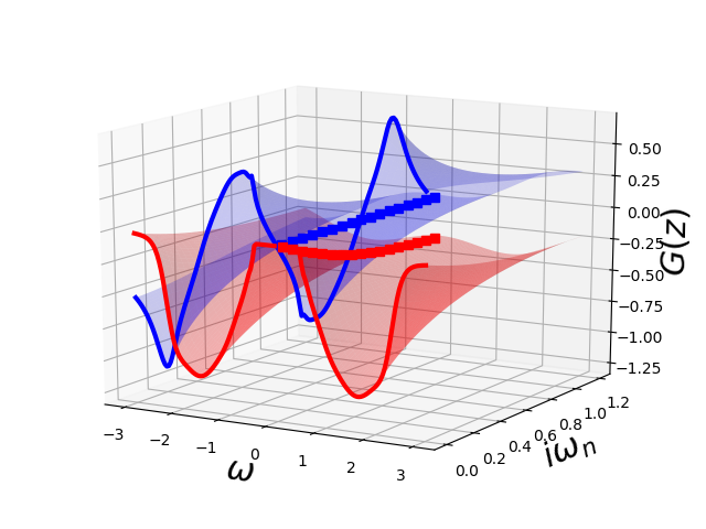
I find it totally surprising how much information is contained in each version of the Greens function and how it forces the complete structure to obey it.

Total running time of the script: ( 0 minutes 6.411 seconds)