Evolution of DOS as function of temperature

Using a real frequency solver in the IPT scheme the Density of states is tracked through the first orders transition.

• 
• 
• 
• 
• 
• 

Out:

D:  1.0 tp/U:  0.3 Beta 28.571428571428573
D:  1.0 tp/U:  0.3 Beta 28.571428571428573
D:  0.2857142857142857 tp/U:  0.12 Beta 100
D:  0.2222222222222222 tp/U:  0.12 Beta 100
0.995642763872
0.995643674807
D:  1.0 tp/U:  0.3 Beta 100
0.997769837988
D:  0.4 tp/U:  0.12 Beta 200
0.997773419019
D:  1.0 tp/U:  0.3 Beta 100
D:  1.0 tp/U:  0.33 Beta 100
D:  1.0 tp/U:  0.35 Beta 100
0.996790151941
0.996117218987
0.995633315986
0.996790151941
0.996117218987
D:  0.3333333333333333 tp/U:  0.1 Beta 250
D:  0.3333333333333333 tp/U:  0.12 Beta 250
D:  0.37037037037037035 tp/U:  0.12 Beta 250
0.999643433571
0.999643440916
0.999643425382

# Created Tue Jun 14 15:44:38 2016
# Author: Óscar Nájera

from __future__ import division, absolute_import, print_function

import numpy as np
import scipy.signal as signal
from scipy.integrate import trapz
import matplotlib.pyplot as plt
from joblib import Parallel, delayed

import dmft.common as gf
import dmft.ipt_real as ipt
from dmft.utils import optical_conductivity

from slaveparticles.quantum.operators import fermi_dist
import slaveparticles.quantum.dos as dos

plt.matplotlib.rcParams.update({'axes.labelsize': 22,
                                'xtick.labelsize': 14, 'ytick.labelsize': 14,
                                'axes.titlesize': 22})


def loop_bandwidth(w, simval, beta, seed='mott gap'):
    """Solves IPT dimer and return Im Sigma_AA, Re Simga_AB

    returns list len(betarange) x 2 Sigma arrays
"""

    s = []
    g = []
    dw = w[1] - w[0]
    gss = gf.semi_circle_hiltrans(w + 5e-3j - 1.3)
    gsa = gf.semi_circle_hiltrans(w + 5e-3j + 1.3)
    nfp = dos.fermi_dist(w, beta)
    for U, D, tp in simval:
        print('D: ', D, 'tp/U: ', tp, 'Beta', beta)
        (gss, gsa), (ss, sa) = ipt.dimer_dmft(
            U, tp, nfp, w, dw, gss, gsa, conv=1e-4, t=(D / 2))
        g.append((gss, gsa))
        s.append((ss, sa))

    return np.array(g), np.array(s), nfp


def plot_spectralfunc(w, gwi, simval, rf, yshift=False):
    shift = 0
    for (gss, gsa), (U, D, tp), r in zip(gwi, simval, rf):
        Awloc = -.5 * (gss + gsa).imag / np.pi
        print(trapz(Awloc, w))
        plt.plot(w, r * Awloc, label=r'U, {}D={:.2},tp={}'.format(U, D, tp))
        #plt.plot(w,  Awloc * nfp, 'k:')

    plt.xlabel(r'$\omega$')
    plt.ylabel(r'$A(\omega)$')
    plt.legend(loc=0)
    plt.xlim([-4, 4])

w = np.linspace(-6, 6, 2**13)
simvals = [(3.5, 1., .3), (4.5, 1., .3)]
giw, swi, nfp = loop_bandwidth(w, simvals, 100 / 3.5)
plt.figure()
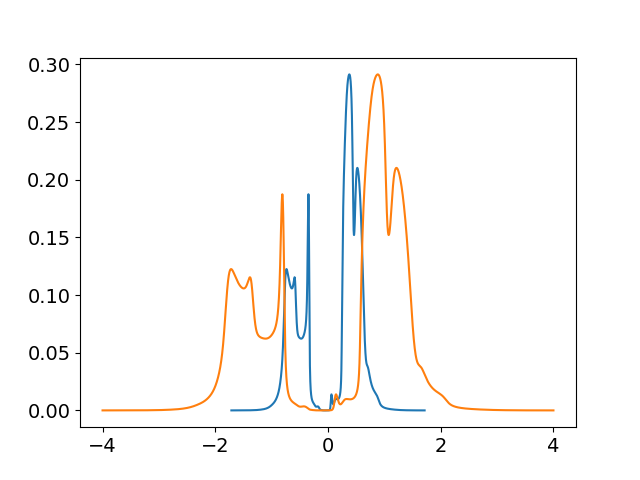
plt.plot(w / 3.5, -.5 * (giw[0][0]).imag / np.pi)
plt.plot(w / 1.5, -.5 * (giw[0][0]).imag / np.pi)

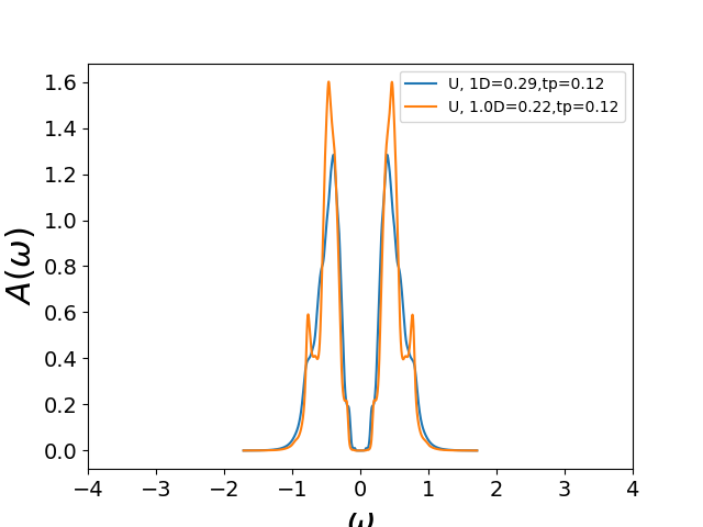
simvals = [(1, 1. / 3.5, .12), (1., 1. / 4.5, .12)]
giw, swi,  nfp = loop_bandwidth(w / 3.5, simvals, 100)
plt.figure()
plot_spectralfunc(w / 3.5, giw, simvals, np.ones(len(simvals)))
plt.figure()
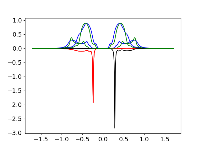
plt.plot(w / 3.5, -.5 * (giw[0][0]).imag / np.pi / 1.14, 'b-')
plt.plot(w / 3.5, .5 * (swi[0][0]).imag / np.pi / 1.14, 'r-')
plt.plot(w / 3.5, .5 * (swi[0][0]).imag / np.pi / 1.14, 'r-')
plt.plot(w / 3.5, -.5 * (giw[0][1]).imag / np.pi / 1.14, 'b-')
plt.plot(w / 3.5, .5 * (swi[1][1]).imag / np.pi / 1.14, 'k-')
plt.plot(w / 3.5, -.5 * (giw[1][0]).imag / np.pi / 1.45, 'g-')
plt.plot(w / 3.5, -.5 * (giw[1][1]).imag / np.pi / 1.45, 'g-')

plt.figure()
simvals = [(2.5, 1., .3)]
giw, swi, nfp = loop_bandwidth(w, simvals, 100)
plot_spectralfunc(w, giw, simvals, np.ones(len(simvals)))

simvals = [(1, 1. / 2.5, .3 / 2.5)]
giw, swi, nfp = loop_bandwidth(w / 2.5, simvals, 200)
plot_spectralfunc(w, giw / 2.5, simvals, np.ones(len(simvals)))

# plt.figure()
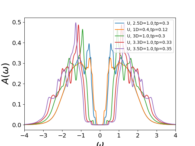
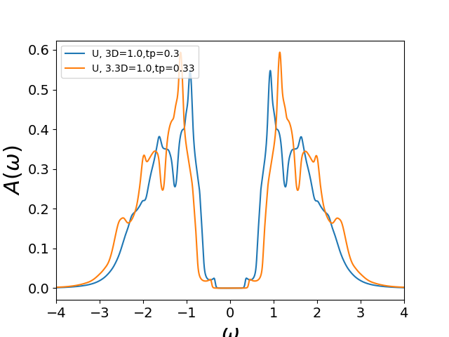
simvals = [(3, 1., .3), (3.3, 1., .33), (3.5, 1., .35)]
giw, swi, nfp = loop_bandwidth(w, simvals, 100)
plot_spectralfunc(w, giw, simvals, np.ones(len(simvals)))

renorm = [1. / .88, 1 / .85, 1 / .82]
renorm = [1 / .85, 1 / .82]
plt.figure()
plot_spectralfunc(w, giw, simvals, renorm)

plt.figure()
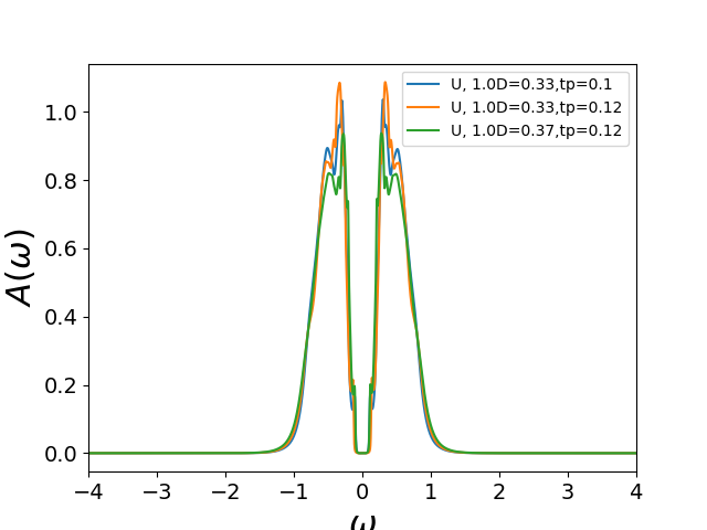
simvals = [(1., 1 / 3., .1), (1., 1 / 3., .12), (1., 1 / 2.7, .12)]
giw, swi, nfp = loop_bandwidth(w, simvals, 250)
plot_spectralfunc(w, giw, simvals, np.ones(len(simvals)))

Total running time of the script: ( 0 minutes 3.602 seconds)