Hubbard III for dimer¶

Describing the position of the Self-Energy pole in the diagonal basis

# Created Mon Mar 14 13:56:37 2016
# Author: Óscar Nájera
from __future__ import absolute_import, division, print_function

import matplotlib.pyplot as plt
import numpy as np

import dmft.common as gf
import dmft.dimer as dimer
from dmft.plot import plot_band_dispersion
import slaveparticles.quantum.operators as op

The Dimer limit¶

Here I study the shape of spectral function and the origin of its poles looking for the zeros of the self energy

def molecule_sigma_d(omega, U, mu, tp, beta):
    """Return molecule self-energy in the given frequency axis"""

    h_at, oper = dimer.hamiltonian_diag(U, mu, tp)
    oper_pair = [[oper[0], oper[0]], [oper[1], oper[1]]]

    eig_e, eig_v = op.diagonalize(h_at.todense())
    gfsU = np.array([op.gf_lehmann(eig_e, eig_v, c.T, beta, omega, d)
                     for c, d in oper_pair])

    plt.plot(omega.real, -(gfsU[1]).imag, label='Anti-Bond')
    plt.plot(omega.real, -(gfsU[0]).imag, label='Bond')
    plt.xlabel(r'$\omega$')
    plt.ylabel(r'$A(\omega)$')
    plt.title(r'Isolated dimer $U={}$, $t_\perp={}$, $\beta={}$'.format(U, tp, beta))
    plt.legend(loc=0)

    return [omega + tp - 1 / gfsU[0], omega - tp - 1 / gfsU[1]]


w = np.linspace(-3, 3, 800)
U = 2.5
tp = 0.3


plt.figure()
sig_b, sig_a = molecule_sigma_d(w + 5e-2j, U, 0, tp, 500)
plt.plot(w, sig_a.real - w + tp, label=r'$\Sigma_{A} - w + t_\perp$')
plt.plot(w, sig_b.real - w - tp, label=r'$\Sigma_{B} - w - t_\perp$')
plt.legend(loc=0)

../_images/sphx_glr_plot_hubbard_III_001.png

Hubbard III approximation¶

Taking advantage of the rotated basis which is diagonal I can independently treat each system on its own and solve 2 decoupled system equations.

In this case the poles of the green function are equally weighted, only its position is correct, in comparison to the isolated dimer green function

sp_2 = (U**2 + 16 * tp**2) / 4.
g0_1_a = w - tp + 5e-2j + 2 * tp  # The excitation out of the singlet has
g0_1_b = w + tp + 5e-2j - 2 * tp  # this extra contribution of 2tp

plt.figure()
x = .60
plt.plot(w, -((1 - (1 - 2 * x) * sp_2 / g0_1_a) /
              (g0_1_a - sp_2 / g0_1_a)).imag, label='Anti-bond')
plt.plot(w, -((1 + (1 - 2 * x) * sp_2 / g0_1_b) /
              (g0_1_b - sp_2 / g0_1_b)).imag, label='Bond')
plt.xlabel(r'$\omega$')
plt.ylabel(r'$A(\omega)$')
plt.title(r'Isolated dimer approximation $U={}$, $t_\perp={}$'.format(U, tp))
plt.legend(loc=0)

for i in range(2000):
    g0_1_a = w - tp - .25 * (1 - (1 - 2 * x) * sp_2 /
                             g0_1_a) / (g0_1_a - sp_2 / g0_1_a)
    g0_1_b = w + tp - .25 * (1 + (1 - 2 * x) * sp_2 /
                             g0_1_b) / (g0_1_b - sp_2 / g0_1_b)

../_images/sphx_glr_plot_hubbard_III_002.png

The Self-Energy¶

plt.figure()
sb = sp_2 * ((1 - 2 * x) + 1 / g0_1_b) / (1 + (1 - 2 * x) * sp_2 / g0_1_b)
plt.plot(w, sb.real, label=r"Re Bond")
plt.plot(w, sb.imag, label=r"Im Bond")

sa = sp_2 * (-(1 - 2 * x) + 1 / g0_1_a) / (1 - (1 - 2 * x) * sp_2 / g0_1_a)
plt.plot(w, sa.real, label=r"Re Anti-Bond")
plt.plot(w, sa.imag, label=r"Im Anti-Bond")

plt.ylabel(r'$\Sigma(\omega)$')
plt.xlabel(r'$\omega$')
plt.title(r'$\Sigma(\omega)$ at $U= {}$'.format(U))
plt.legend(loc=0)
plt.ylim([-3.5, 2])

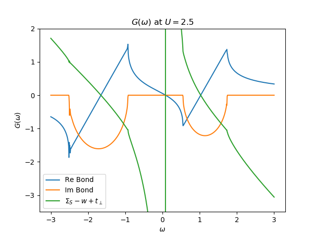
../_images/sphx_glr_plot_hubbard_III_003.png

The Green Function¶

plt.figure()
g_b = 1 / (w + tp - sb)
plt.plot(w, g_b.real, label=r"Re Bond")
plt.plot(w, g_b.imag, label=r"Im Bond")
plt.figure()
g_b = gf.greenF(-1j * w, sb, tp)
zeta = w + tp - sb
g_b = 2 * zeta * (1 - np.sqrt(1 - 1 / zeta**2))
g_b = 1 / (g0_1_b - sb)
plt.plot(w, g_b.real, label=r"Re Bond")
plt.plot(w, g_b.imag, label=r"Im Bond")
plt.plot(w, sb.real - w - tp, label=r'$\Sigma_{S} - w + t_\perp$')

plt.ylabel(r'$G(\omega)$')
plt.xlabel(r'$\omega$')
plt.title(r'$G(\omega)$ at $U= {}$'.format(U))
plt.ylim([-3.5, 2])
plt.legend(loc=0)

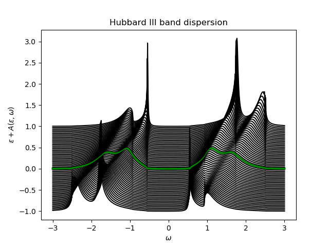
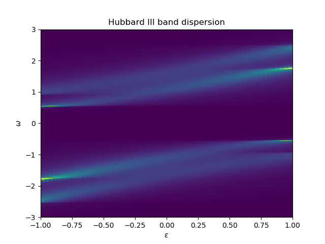
The Band Dispersion¶

eps_k = np.linspace(-1, 1, 61)
lat_gf = 1 / (np.add.outer(-eps_k, w + tp + 8e-2j) - sp_2 / g0_1_b) + \
    1 / (np.add.outer(-eps_k, w - tp + 8e-2j) - sp_2 / g0_1_a)
Aw = -lat_gf.imag / np.pi / 2


plot_band_dispersion(w, Aw, 'Hubbard III band dispersion', eps_k)