Dimer Mott transition Optical response

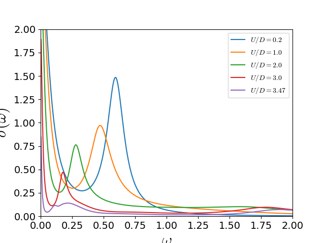
Track the optical conductivity from the correlated metal up to the transition point. The lost of overlap of bonding and anti-bonding bands at the Fermi level implies the transition. From the optical signal the Drude weight drops with raising U and the Inter-band transition signal lowers its excitation energy signaling how the two quasiparticles are renormalized closer together.

See also

Dimer Mott transition The insulator transition order parameter

# author: Óscar Nájera

from __future__ import division, absolute_import, print_function

import numpy as np
import matplotlib.pyplot as plt

import dmft.common as gf
import dmft.ipt_real as ipt
import dmft.dimer as dimer

plt.matplotlib.rcParams.update({'axes.labelsize': 22,
                                'xtick.labelsize': 14, 'ytick.labelsize': 14,
                                'axes.titlesize': 22,
                                'mathtext.fontset': 'cm'})

w = np.linspace(-4, 4, 2**12)
dw = w[1] - w[0]

BETA = 800.
nfp = gf.fermi_dist(w, BETA)

tp = 0.3
gss = gf.semi_circle_hiltrans(w + 5e-3j - tp)
gsa = gf.semi_circle_hiltrans(w + 5e-3j + tp)
urange = np.arange(0.2, 3.3, 0.3)
urange = [0.2, 1., 2., 3., 3.47]
plt.close('all')
eps_k = np.linspace(-1, 1, 61)
pos_freq = w > 0
nuv = w[pos_freq]

for i, U in enumerate(urange):
    (gss, gsa), (ss, sa) = ipt.dimer_dmft(
        U, tp, nfp, w, dw, gss, gsa, conv=1e-4)

    s_intra, s_inter = dimer.optical_conductivity(BETA, ss, sa, w, tp, eps_k)

    ddm_sigma_E_sum = .5 * (s_intra + s_inter)

    shift = -2.1 * i
    plt.plot(nuv, ddm_sigma_E_sum, label=r'$U/D={}$'.format(U))

plt.xlabel(r'$\omega$')
plt.ylabel(r'$\sigma(\omega)$')
plt.xlim(0, 2)
plt.ylim(0, 2)
plt.legend(loc=0)

Total running time of the script: ( 0 minutes 3.529 seconds)