Isolated molecule spectral function 2

For the case of contact interaction in the di-atomic molecule case spectral function are evaluated by means of the Lehmann representation

# author: Óscar Nájera

from __future__ import division, absolute_import, print_function
from itertools import product, combinations
import matplotlib.pyplot as plt
import numpy as np
import scipy.linalg as LA
from dmft.common import matsubara_freq, gw_invfouriertrans
import dmft.dimer as dimer
import slaveparticles.quantum.operators as op

The Dimer alone

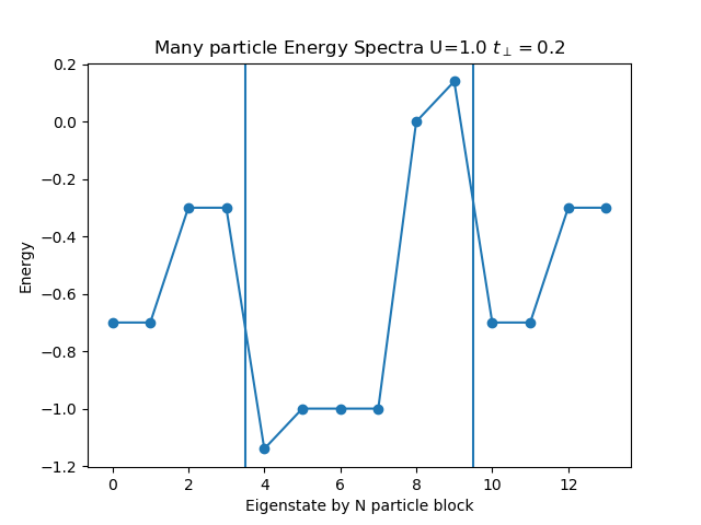
The ground state for half filling is defined at superposition of S=0 states containing the double occupation of each site plus the individually occupied sites. This allows for the super-exchange process and makes it the ground state. The first exited state is formed by the triplet states S=1 where sites are singly occupied

def plot_eigen_spectra(U, mu, tp):
    h_at, oper = dimer.hamiltonian(U, mu, tp)
    eig_e = []
    eig_e.append(LA.eigvalsh(h_at[1:5, 1:5].todense()))
    eig_e.append(LA.eigvalsh(h_at[5:11, 5:11].todense()))
    eig_e.append(LA.eigvalsh(h_at[11:15, 11:15].todense()))

    plt.figure()
    plt.title('Many particle Energy Spectra U={} $t_\perp={}$'.format(U, tp))
    plt.plot(np.concatenate(eig_e), "o-")
    plt.ylabel('Energy')
    plt.xlabel('Eigenstate by N particle block')

    plt.axvline(x=3.5)
    plt.axvline(x=9.5)
plot_eigen_spectra(1., 0, 0.2)

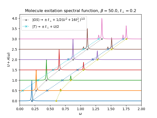
From the next Spectral functions we see that exitations go from ground state to the bonding anti-bonding bands. If the ground-state is close to the triplet state or reachable by thermal exitation, it is also possible to see the exitation from the triplet state to the bonding anti-bonding bands.

The main role in the spetra is played by the local interaction, which is allowed to grow sufficiently. It split the largely the exitation spectra, the inner hopping parameter plays little role, only to lift the ground state degeneracy by super-exchange.

def plot_A_ev_ru(beta, urange, mu, tp):
    w = np.linspace(0, 2, 500) + 1j * 5e-3
    for u_int in urange:
        h_at, oper = dimer.hamiltonian(u_int, mu, tp)
        eig_e, eig_v = op.diagonalize(h_at.todense())
        gf = op.gf_lehmann(eig_e, eig_v, oper[0].T, beta, w)
        plt.plot(w.real, u_int + gf.imag / gf.imag.min())
    plt.plot(0.5 * np.sqrt(urange**2 + 16 * tp**2) - tp, urange, '*:',
             label=r'$|GS\rangle \rightarrow \pm t_\perp + 1/2(U^2+16t^2_\perp)^{1/2}$')
    plt.plot(0.5 * np.sqrt(urange**2 + 16 * tp**2) + tp, urange, '*:')
    plt.plot(urange / 2 - tp, urange, 'x:',
             label=r'$|T\rangle \rightarrow \pm t_\perp + U/2$')
    plt.plot(urange / 2 + tp, urange, 'x:')
    plt.xlim([min(w.real), max(w.real)])
plt.figure()
beta, tp = 50., .2
plot_A_ev_ru(beta, np.arange(0.0, 3.1, 0.5), 0, tp)
plt.title(
    r'Molecule exitation spectral function, $\beta={}$, $t_\perp={}$'.format(beta, tp))
plt.xlabel(r'$\omega$')
plt.ylabel(r'$U+A(\omega)$')
plt.legend(loc=0)


def plot_A_ev_rtp(beta, u_int, mu, tprange):
    w = np.linspace(-4, 4, 5500) + 1j * 5e-3
    for tp in tprange:
        h_at, oper = dimer.hamiltonian(u_int, mu, tp)
        eig_e, eig_v = op.diagonalize(h_at.todense())
        gfd = op.gf_lehmann(eig_e, eig_v, oper[0].T, beta, w)
        gfo = op.gf_lehmann(eig_e, eig_v, oper[0].T, beta, w, oper[1])
        gf = gfd + gfo

        plt.plot(w.real, tp + gf.imag / gf.imag.min())
    plt.title('Molecule exitation spectral function')
    plt.xlabel(r'$\omega$')
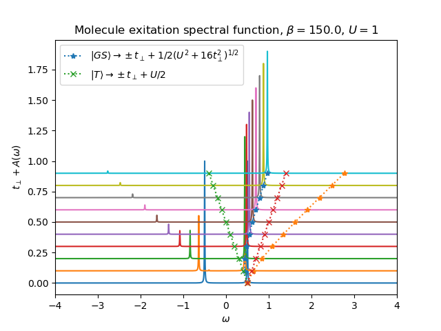
    plt.plot(0.5 * np.sqrt(u_int**2 + 16 * tprange**2) - tprange, tprange, '*:',
             label=r'$|GS\rangle \rightarrow \pm t_\perp + 1/2(U^2+16t^2_\perp)^{1/2}$')
    plt.plot(0.5 * np.sqrt(u_int**2 + 16 * tprange**2) + tprange, tprange, '*:')
    plt.plot(u_int / 2 - tprange, tprange, 'x:',
             label=r'$|T\rangle \rightarrow \pm t_\perp + U/2$')
    plt.plot(u_int / 2 + tprange, tprange, 'x:')
    plt.xlim([min(w.real), max(w.real)])

plt.figure()
beta, U = 150., 1
plot_A_ev_rtp(beta, 1, 0, np.arange(0.0, 1, 0.1))
plt.title(r'Molecule exitation spectral function, $\beta={}$, $U={}$'.format(beta, U))
plt.xlabel(r'$\omega$')
plt.ylabel(r'$t_\perp+A(\omega)$')
plt.legend(loc=0)


def plot_A_ev_utp(beta, urange, mu, tprange):
    w = np.linspace(-2, 2, 1500) + 1j * 5e-3
    for u_int, tp in zip(urange, tprange):
        h_at, oper = dimer.hamiltonian(u_int, mu, tp)
        eig_e, eig_v = op.diagonalize(h_at.todense())
        gf = op.gf_lehmann(eig_e, eig_v, oper[0].T, beta, w)
        plt.plot(w.real, u_int + gf.imag / gf.imag.min(), 'k-')

plt.figure()
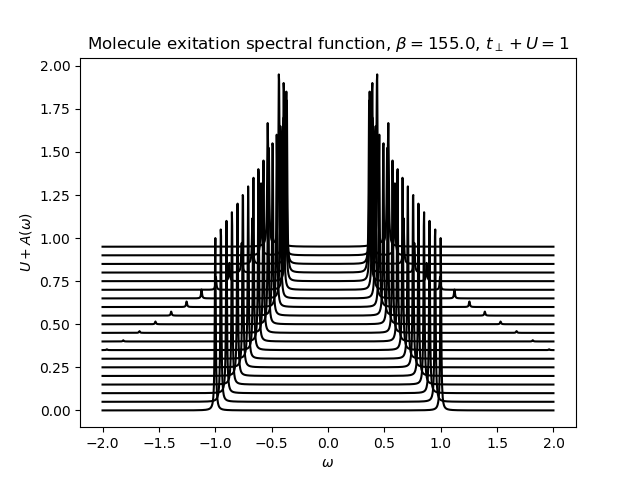
beta, tp = 155., .2
plot_A_ev_utp(beta, np.arange(0.0, 1, 0.05), 0, np.arange(1, 0, -0.05))
plt.title(
    r'Molecule exitation spectral function, $\beta={}$, $t_\perp+U=1$'.format(beta))
plt.xlabel(r'$\omega$')
plt.ylabel(r'$U+A(\omega)$')
plt.legend(loc=0)

• 
• 
• 

Diagonal basis

def plot_A_ev_utp(beta, urange, mu, tprange):
    w = np.linspace(-2, 3.5, 1500) + 1j * 1e-2
    Aw = []
    for u_int, tp in zip(urange, tprange):
        h_at, oper = dimer.hamiltonian_diag(u_int, mu, tp)
        eig_e, eig_v = op.diagonalize(h_at.todense())
        gf = op.gf_lehmann(eig_e, eig_v, oper[0].T, beta, w)
        aw = gf.imag / gf.imag.min()
        Aw.append(aw)
    return np.array(Aw)

beta = 100.
A = plot_A_ev_utp(beta, np.linspace(0, 1, 51), 0, np.linspace(0, 1, 51)[::-1])

w = np.linspace(-2, 3.5, 1500)
#plot_band_dispersion(w, A, r'Molecule exitation spectral function, $\beta={}$, $t_\perp+U=1$'.format(beta), np.linspace(0, 1, 51))
plt.figure(1)
plt.ylabel(r'$U+A(\omega)$')
plt.xlim([-2, 3.5])
plt.figure(2)
plt.xlabel(r'$\omega$')
plt.ylabel(r'$U$')
plt.ylim([-2, 3.5])

• 
• 

Total running time of the script: ( 0 minutes 2.263 seconds)