Evolution of DOS as function of temperature

Using a real frequency solver in the IPT scheme the Density of states is tracked through the first orders transition.

Out:

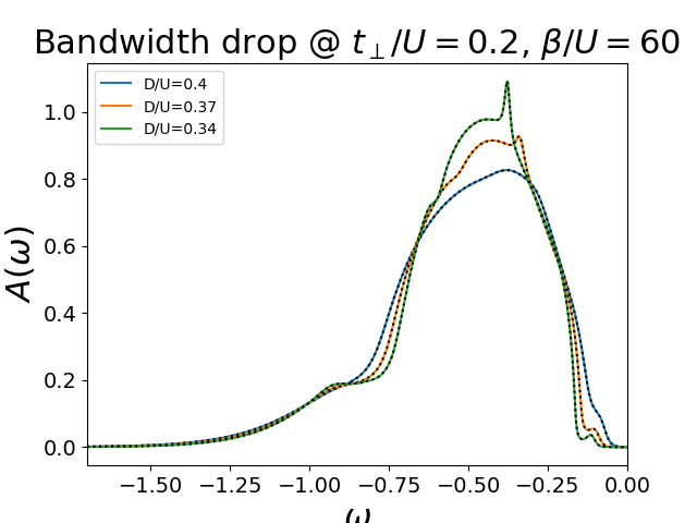
D/U:  0.4 tp/U:  0.2 Beta 60
D/U:  0.37037037037 tp/U:  0.2 Beta 60
D/U:  0.344827586207 tp/U:  0.2 Beta 60
0.999643296063
0.999643302756
0.999643308605

# Created Tue Jun 14 15:44:38 2016
# Author: Óscar Nájera

from __future__ import division, absolute_import, print_function

import numpy as np
import scipy.signal as signal
from scipy.integrate import trapz
import matplotlib.pyplot as plt
from joblib import Parallel, delayed

import dmft.common as gf
import dmft.ipt_real as ipt
from dmft.utils import optical_conductivity

plt.matplotlib.rcParams.update({'axes.labelsize': 22,
                                'xtick.labelsize': 14, 'ytick.labelsize': 14,
                                'axes.titlesize': 22})


def loop_bandwidth(drange, tp, beta, seed='mott gap'):
    """Solves IPT dimer and return Im Sigma_AA, Re Simga_AB

    returns list len(betarange) x 2 Sigma arrays
"""

    s = []
    g = []
    w = np.linspace(-6, 6, 2**13)
    dw = w[1] - w[0]
    gssi = gf.semi_circle_hiltrans(w + 5e-3j - tp - 1)
    gsai = gf.semi_circle_hiltrans(w + 5e-3j + tp + 1)
    nfp = gf.fermi_dist(w, beta)
    for D in drange:
        print('D/U: ', D, 'tp/U: ', tp, 'Beta', beta)
        (gss, gsa), (ss, sa) = ipt.dimer_dmft(
            1, tp, nfp, w, dw, gssi, gssi, conv=1e-2, t=(D / 2))
        g.append((gss, gsa))
        s.append((ss, sa))

    return np.array(g), np.array(s), w, nfp


def plot_spectralfunc(gwi, drange, yshift=False):
    plt.figure()
    shift = 0
    for (gss, gsa), D in zip(gwi, drange):
        Awloc = -.5 * (gss + gsa).imag / np.pi
        print(trapz(Awloc, w))
        plt.plot(w,  Awloc, label=r'D/U={:.2}'.format(D))
        plt.plot(w,  Awloc * nfp, 'k:')

    plt.xlabel(r'$\omega$')
    plt.ylabel(r'$A(\omega)$')
    plt.legend(loc=0)
    plt.xlim([-1.7, 0])

drange = 1 / np.array([2.5, 2.7, 2.9])
giw, swi, w, nfp = loop_bandwidth(drange, 0.2, 60)
plot_spectralfunc(giw, drange)
plt.title(r"Bandwidth drop @ $t_\perp/U=0.2$, $\beta/U=60$")

#giw, swi, w, nfp = loop_bandwidth(drange, 0.3, 180)
#plot_spectralfunc(giw, drange)
#plt.title(r"Bandwidth drop @ $t_\perp/U=0.17$, $\beta/U=150$")

Total running time of the script: ( 0 minutes 0.823 seconds)