Non-interacting atom under external field spectral function

An Isolated atom with non-interacting electrons is set under the influence of an external magnetic field

• 
• 

# author: Óscar Nájera

from __future__ import division, absolute_import, print_function
import numpy as np
import matplotlib.pyplot as plt
from dmft.common import matsubara_freq
from slaveparticles.quantum import fermion
from slaveparticles.quantum.operators import gf_lehmann, diagonalize


def hamiltonian(M, mu):
    r"""Generate a single orbital isolated atom Hamiltonian in particle-hole
    symmetry. Include chemical potential for grand Canonical calculations

    .. math::
        \mathcal{H} - \mu N = M(n_\uparrow - n_\downarrow)
        - \mu(n_\uparrow + n_\downarrow)

    """
    d_up, d_dw = [fermion.destruct(2, sigma) for sigma in range(2)]
    sigma_z = d_up.T*d_up - d_dw.T*d_dw
    H = M * sigma_z - mu * (d_up.T*d_up + d_dw.T*d_dw)
    return H, d_up, d_dw


def gf(w, U, mu, beta):
    """Calculate by Lehmann representation the green function"""
    H, d_up, d_dw = hamiltonian(U, mu)
    e, v = diagonalize(H.todense())
    g_up = gf_lehmann(e, v, d_up.T, beta, w)
    g_dw = gf_lehmann(e, v, d_dw.T, beta, w)
    return g_up, g_dw


beta = 50
M = 0.5
mu_v = np.array([0, 0.2, 0.45, 0.5, 0.65])
c_v = ['b', 'g', 'r', 'k', 'm']

f, axw = plt.subplots(2, sharex=True)
f.subplots_adjust(hspace=0)
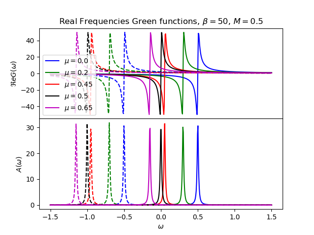
w = np.linspace(-1.5, 1.5, 500) + 1j*1e-2
for mu, c in zip(mu_v, c_v):
    gws = gf(w, M, mu, beta)
    for gw in gws:
        first = np.allclose(gw, gws[0])
        axw[0].plot(w.real, gw.real, c if first else c+'--',
                    label=r'$\mu={}$'.format(mu) if first else None)
        axw[1].plot(w.real, -1*gw.imag/np.pi, c if first else c+'--')
axw[0].legend()
axw[0].set_title(r'Real Frequencies Green functions, $\beta={}$, $M={}$'.format(beta, M))
axw[0].set_ylabel(r'$\Re e G(\omega)$')
axw[1].set_ylabel(r'$A(\omega)$')
axw[1].set_xlabel(r'$\omega$')


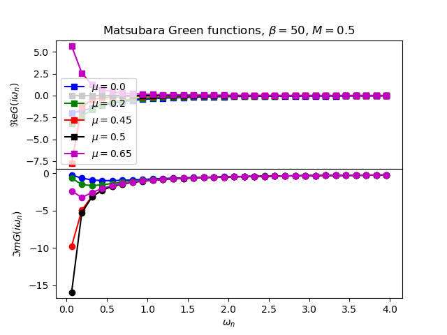
g, axwn = plt.subplots(2, sharex=True)
g.subplots_adjust(hspace=0)
wn = matsubara_freq(beta, 32)
for mu, c in zip(mu_v, c_v):
    giw = gf(1j*wn, M, mu, beta)[0]
    axwn[0].plot(wn, giw.real, c+'s-', label=r'$\mu={}$'.format(mu))
    axwn[1].plot(wn, giw.imag, c+'o-')
axwn[0].legend()
axwn[0].set_title(r'Matsubara Green functions, $\beta={}$, $M={}$'.format(beta, M))
axwn[1].set_xlabel(r'$\omega_n$')
axwn[0].set_ylabel(r'$\Re e G(i\omega_n)$')
axwn[1].set_ylabel(r'$\Im m G(i\omega_n)$')

Total running time of the script: ( 0 minutes 0.344 seconds)