Interacting atom spectral function

For the case of contact interaction in the single orbital case the atomic Green function as given by the Lehmann Representation.

• 
• 
• 

# author: Óscar Nájera

from __future__ import division, absolute_import, print_function
import numpy as np
import matplotlib.pyplot as plt
from dmft.common import matsubara_freq, gw_invfouriertrans
from slaveparticles.quantum import fermion
from slaveparticles.quantum.operators import gf_lehmann, diagonalize


def hamiltonian(U, mu):
    r"""Generate a single orbital isolated atom Hamiltonian in particle-hole
    symmetry. Include chemical potential for grand Canonical calculations

    .. math::
        \mathcal{H} - \mu N = -\frac{U}{2}(n_\uparrow - n_\downarrow)^2
        - \mu(n_\uparrow + n_\downarrow)

    """
    d_up, d_dw = [fermion.destruct(2, sigma) for sigma in range(2)]
    sigma_z = d_up.T * d_up - d_dw.T * d_dw
    H = - U / 2 * sigma_z * sigma_z - mu * (d_up.T * d_up + d_dw.T * d_dw)
    return H, d_up, d_dw


def gf(w, U, mu, beta):
    """Calculate by Lehmann representation the green function"""
    H, d_up, d_dw = hamiltonian(U, mu)
    e, v = diagonalize(H.todense())
    g_up = gf_lehmann(e, v, d_up.T, beta, w)
    return g_up


beta = 50
U = 1.
mu_v = np.array([0, 0.2, 0.45, 0.5, 0.65])
c_v = ['b', 'g', 'r', 'k', 'm']

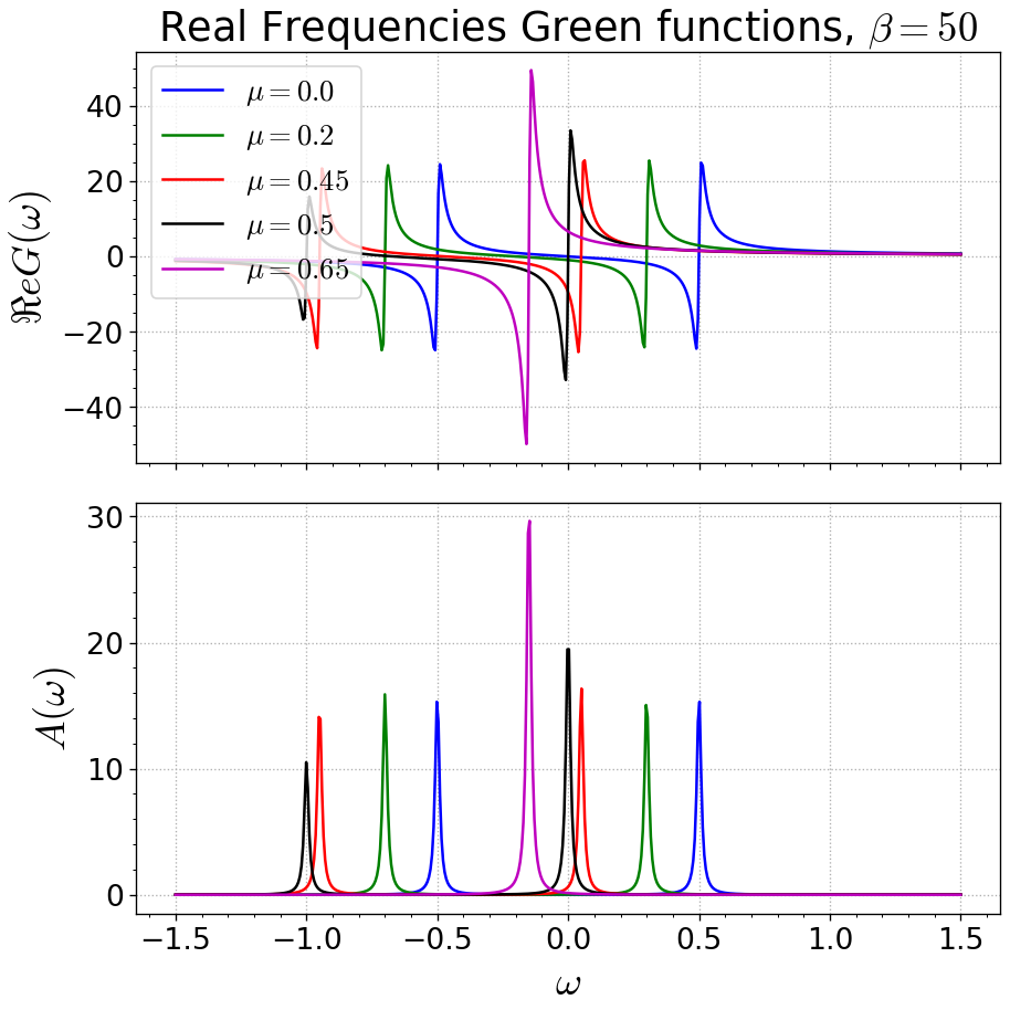
f, axw = plt.subplots(2, sharex=True)
f.subplots_adjust(hspace=0)
w = np.linspace(-1.5, 1.5, 500) + 1j * 1e-2
for mu, c in zip(mu_v, c_v):
    gw = gf(w, U, mu, beta)
    axw[0].plot(w.real, gw.real, c, label=r'$\mu={}$'.format(mu))
    axw[1].plot(w.real, -1 * gw.imag / np.pi, c)
axw[0].legend()
axw[0].set_title(r'Real Frequencies Green functions, $\beta={}$'.format(beta))
axw[0].set_ylabel(r'$\Re e G(\omega)$')
axw[1].set_ylabel(r'$A(\omega)$')
axw[1].set_xlabel(r'$\omega$')


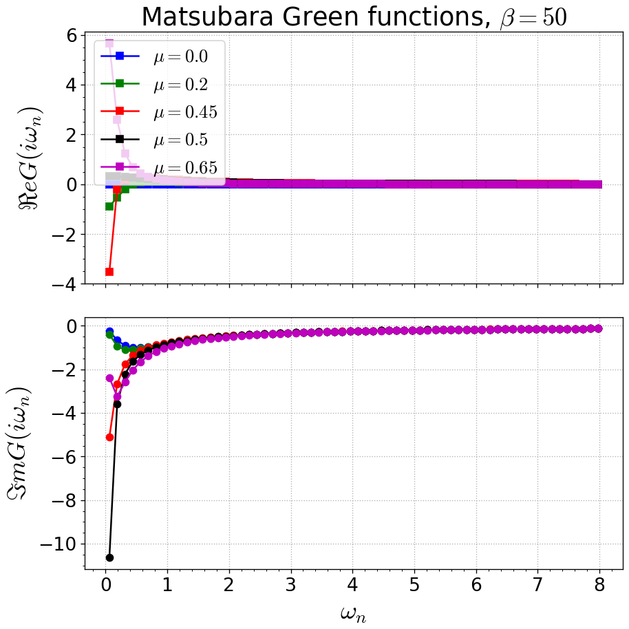
gwp, axwn = plt.subplots(2, sharex=True)
gwp.subplots_adjust(hspace=0)
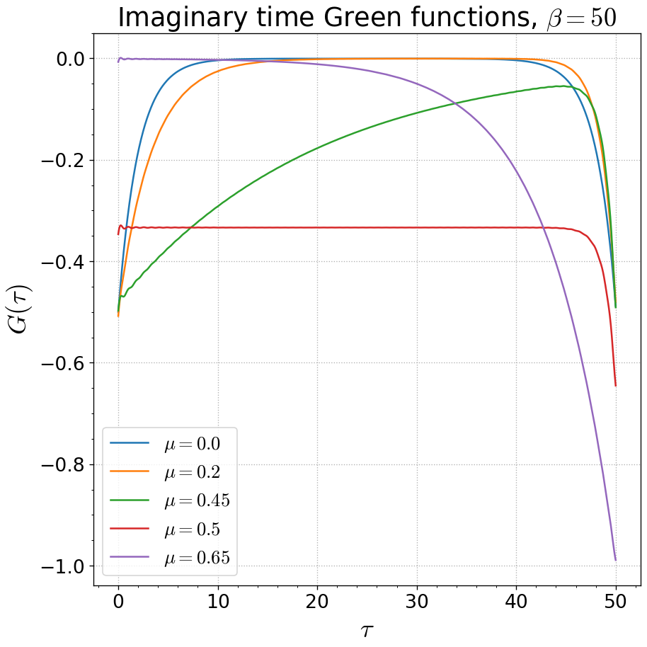
gtp, axt = plt.subplots()
wn = matsubara_freq(beta, 64)
tau = np.linspace(0, beta, 2**10)
for mu, c in zip(mu_v, c_v):
    giw = gf(1j * wn, U, mu, beta)
    axwn[0].plot(wn, giw.real, c + 's-', label=r'$\mu={}$'.format(mu))
    axwn[1].plot(wn, giw.imag, c + 'o-')

    gt = gw_invfouriertrans(giw, tau, wn)
    axt.plot(tau, gt, label=r'$\mu={}$'.format(mu))

axwn[0].legend()
axwn[0].set_title(r'Matsubara Green functions, $\beta={}$'.format(beta))
axwn[1].set_xlabel(r'$\omega_n$')
axwn[0].set_ylabel(r'$\Re e G(i\omega_n)$')
axwn[1].set_ylabel(r'$\Im m G(i\omega_n)$')

axt.set_ylim(top=0.05)
axt.legend(loc=0)
axt.set_title(r'Imaginary time Green functions, $\beta={}$'.format(beta))
axt.set_xlabel(r'$\tau$')
axt.set_ylabel(r'$G(\tau)$')

Total running time of the script: ( 0 minutes 0.531 seconds)