Hubbard I for dimer diagonal basis¶

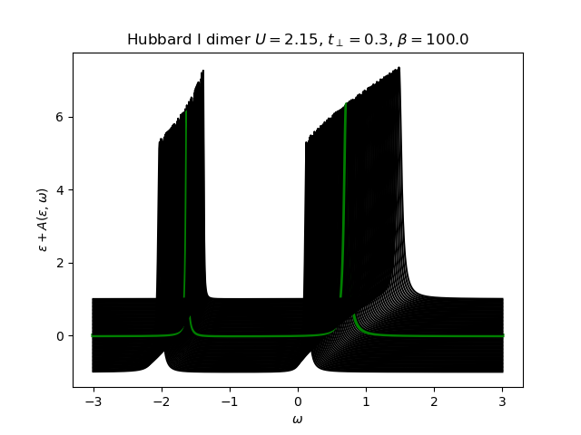
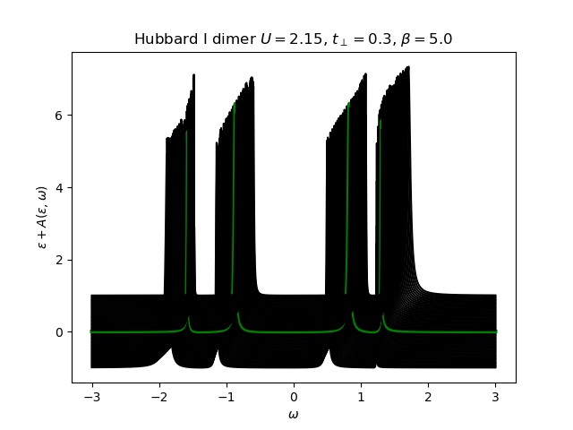
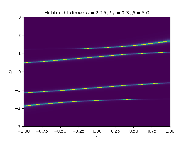
The atomic self-energy is extracted and plotted into the lattice Green’s function to see the behavior of the insulating state. Use the anti-bonding function

# Created Mon Mar 14 13:56:37 2016
# Author: Óscar Nájera

from __future__ import division, absolute_import, print_function

import matplotlib.pyplot as plt
import numpy as np
from dmft.common import gw_invfouriertrans
from dmft.plot import plot_band_dispersion
import dmft.dimer as dimer
import slaveparticles.quantum.operators as op

Approximating Hubbard I¶

Here I use the molecule self-energy

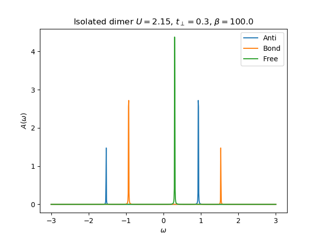
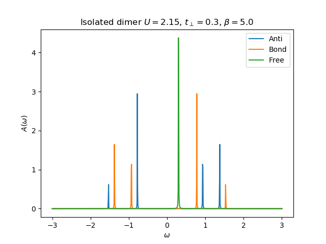
def molecule_sigma(omega, U, mu, tp, beta):
    """Return molecule self-energy in the given frequency axis"""

    h_at, oper = dimer.hamiltonian_diag(U, mu, tp)
    oper_pair = [[oper[1], oper[1]], [oper[0], oper[0]]]

    eig_e, eig_v = op.diagonalize(h_at.todense())
    gfsU = np.array([op.gf_lehmann(eig_e, eig_v, c.T, beta, omega, d)
                     for c, d in oper_pair])

    plt.plot(omega.real, -gfsU[0].imag, label='Anti')
    plt.plot(omega.real, -gfsU[1].imag, label='Bond')
    plt.plot(omega.real, -(1 / (omega - tp)).imag, label='Free')
    plt.xlabel(r'$\omega$')
    plt.ylabel(r'$A(\omega)$')
    plt.title(r'Isolated dimer $U={}$, $t_\perp={}$, $\beta={}$'.format(U, tp, beta))
    plt.legend(loc=0)

    return [omega - tp - 1 / gfsU[0], omega + tp - 1 / gfsU[1]]

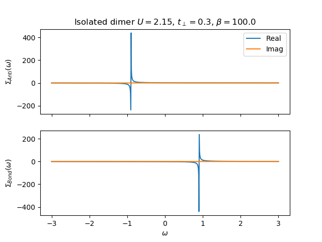
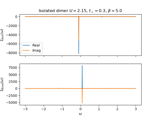
The Real axis Self-energy¶

def plot_self_energy(w, sd_w, so_w, U, mu, tp, beta):
    f, ax = plt.subplots(2, sharex=True)
    ax[0].plot(w, sd_w.real, label='Real')
    ax[0].plot(w, sd_w.imag, label='Imag')
    ax[1].plot(w, so_w.real, label='Real')
    ax[1].plot(w, so_w.imag, label='Imag')
    ax[0].legend(loc=0)
    ax[1].set_xlabel(r'$\omega$')
    ax[0].set_ylabel(r'$\Sigma_{Anti}(\omega)$')
    ax[1].set_ylabel(r'$\Sigma_{Bond}(\omega)$')
    ax[0].set_title(
        r'Isolated dimer $U={}$, $t_\perp={}$, $\beta={}$'.format(U, tp, beta))

w = np.linspace(-3, 3, 800)
U, mu, tp, beta = 2.15, 0., 0.3, 100.
sd_w, so_w = molecule_sigma(w + 5e-5j, U, mu, tp, beta)
plot_self_energy(w, sd_w, so_w, U, mu, tp, beta)

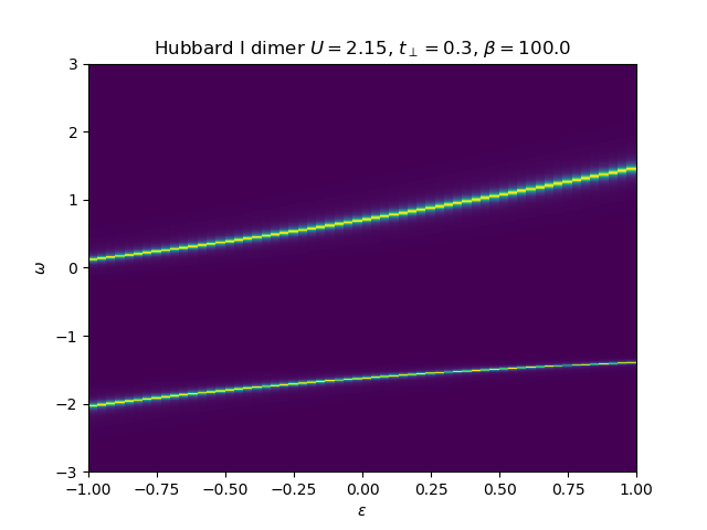
Hubbard I Band dispersion¶

eps_k = np.linspace(-1, 1, 61)
lat_gf = 1 / np.add.outer(-eps_k, w + 5e-2j - sd_w)
Aw = -lat_gf.imag / np.pi

plot_band_dispersion(
    w, Aw, r'Hubbard I dimer $U={}$, $t_\perp={}$, $\beta={}$'.format(U, tp, beta), eps_k)

The Real axis Self-energy¶

w = np.linspace(-3, 3, 800)
U, mu, tp, beta = 2.15, 0., 0.3, 5.
sd_w, so_w = molecule_sigma(w + 5e-5j, U, mu, tp, beta)
plot_self_energy(w, sd_w, so_w, U, mu, tp, beta)

Hubbard I Band dispersion¶

eps_k = np.linspace(-1, 1, 61)
lat_gf = 1 / np.add.outer(-eps_k, w + 5e-2j - sd_w)
Aw = -lat_gf.imag / np.pi
plot_band_dispersion(
    w, Aw, r'Hubbard I dimer $U={}$, $t_\perp={}$, $\beta={}$'.format(U, tp, beta), eps_k)