Comparing the effect of disorder

# Author: Óscar Nájera

from __future__ import (absolute_import, division, print_function,
                        unicode_literals)

import matplotlib.pyplot as plt
import numpy as np

import dmft.common as gf
import dmft.ipt_imag as ipt
from dmft.ipt_real import dimer_dmft as dimer_dmft_real
import dmft.dimer as dimer
from slaveparticles.quantum import dos


def plot_gf(gw, sw, axes):
    axes[0].plot(w, -gw.imag / np.pi)
    axes[1].plot(w, sw.real)
    axes[1].axhline(0, color='k')
    axes[2].plot(w, -sw.imag)

Insulator in IPT Imag local basis

def dmft_solve(giw_d, giw_o, beta, u_int, tp, tau, w_n):
    giw_d, giw_o, loops = dimer.ipt_dmft_loop(
        BETA, u_int, tp, giw_d, giw_o, tau, w_n, 1e-12)
    g0iw_d, g0iw_o = dimer.self_consistency(
        1j * w_n, 1j * giw_d.imag, giw_o.real, 0., tp, 0.25)
    siw_d, siw_o = ipt.dimer_sigma(u_int, tp, g0iw_d, g0iw_o, tau, w_n)
    return giw_d, giw_o, siw_d, siw_o


plt.close('all')
u_int = 2.65
BETA = 100.

tau, w_n = gf.tau_wn_setup(dict(BETA=BETA, N_MATSUBARA=1024))
giw_d, giw_o = 1 / (1j * w_n + 4j / w_n), np.zeros_like(w_n) + 0j
w = np.linspace(-4, 4, 2**13 + 1)


giw_dt0, giw_ot0, siw_dt0, siw_ot0 = dmft_solve(
    giw_d, giw_o, BETA, u_int, 0, tau, w_n)

giw_dt03, giw_ot03, siw_dt03, siw_ot03 = dmft_solve(
    giw_d, giw_o, BETA, u_int, 0.3, tau, w_n)

Disorder comparison plots

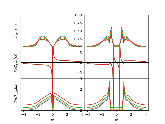
There is a transfer of spectral weight out of the Hubbard bands. The maxima drop by about 40% in fraction, but in magnitude the melting of the peak is much more drastic.

w_set = np.concatenate((np.arange(80), np.arange(80, 150, 5)))
gwst0 = gf.pade_continuation(1j * giw_dt0.imag + giw_ot0.real, w_n, w, w_set)
swst0 = gf.pade_continuation(1j * siw_dt0.imag + siw_ot0.real, w_n, w, w_set)
gwst03 = gf.pade_continuation(
    1j * giw_dt03.imag + giw_ot03.real, w_n, w, w_set)
swst03 = gf.pade_continuation(
    1j * siw_dt03.imag + siw_ot03.real, w_n, w, w_set)


fig, axes = plt.subplots(3, 2, sharex=True)
fig.subplots_adjust(hspace=0, wspace=0.0)

for gamma in [0, 0.1, .25, .5]:
    swt0 = swst0.real - 1j * np.abs(swst0.imag) - gamma * 1j
    swt03 = swst03.real - 1j * np.abs(swst03.imag) - gamma * 1j

    plot_gf(gf.semi_circle_hiltrans(w - swt0), swt0, axes[:, 0])

    gf03 = gf.semi_circle_hiltrans(w - 0.3 - swt03)
    gf03 = .5 * (gf03 + gf03[::-1])

    sst03 = .5 * (swt03 - swt03[::-1].conj())
    plot_gf(gf03, sst03, axes[:, 1])

axes[0, 0].set_ylabel(r'$A_{sym}(\omega)$')
axes[1, 0].set_ylabel(r'$\Re e \Sigma_{sym}(\omega)$')
axes[2, 0].set_ylabel(r'$-\Im m \Sigma_{sym}(\omega)$')

for ax, lim in zip(axes, [[0, 1], [-8, 8], [0, 3]]):
    ax[0].set_ylim(lim)
    ax[0].set_yticks([])
    ax[1].set_ylim(lim)


axes[2, 0].set_xlabel(r'$\omega$')
axes[2, 1].set_xlabel(r'$\omega$')

Total running time of the script: ( 0 minutes 1.207 seconds)