Hubbard III approximation

In this approach the aim is to find the band dispersion of the insulating system but including the effects of the bath. For this one approximates the local Green’s function by

And the using the self consistency equation of the Bethe lattice

Here this equation can be solved analytically but for current purposes

here it will be solved by fixed point iteration.

# Created Fri Apr  1 14:44:59 2016
# Author: Óscar Nájera

from __future__ import absolute_import, division, print_function

import numpy as np
import matplotlib.pyplot as plt

import dmft.common as gf
from dmft.plot import plot_band_dispersion


w = np.linspace(-3, 3, 800)
g0_1 = w + 1e-6j
U = 2.

for i in range(2000):
    g0_1 = w - .25 / (g0_1 - U**2 / 4. / g0_1)

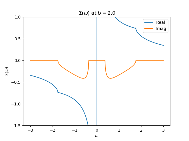
The Self-Energy

plt.figure()
plt.plot(w, (U**2 / 4 / g0_1).real, label=r"Real")
plt.plot(w, (U**2 / 4 / g0_1).imag, label=r"Imag")

plt.ylabel(r'$\Sigma(\omega)$')
plt.xlabel(r'$\omega$')
plt.title(r'$\Sigma(\omega)$ at $U= {}$'.format(U))
plt.legend(loc=0)
plt.ylim([-1.5, 1])

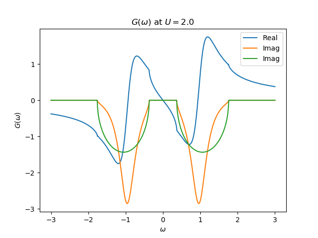
The Green Function

plt.figure()
plt.plot(w, (1 / (w - U**2 / 4 / g0_1)).real, label=r"Real")
plt.plot(w, (1 / (w - U**2 / 4 / g0_1)).imag, label=r"Imag")
plt.plot(w, (gf.semi_circle_hiltrans(w - U**2 / 4 / g0_1)).imag, label=r"Imag")

plt.ylabel(r'$G(\omega)$')
plt.xlabel(r'$\omega$')
plt.title(r'$G(\omega)$ at $U= {}$'.format(U))
plt.legend(loc=0)

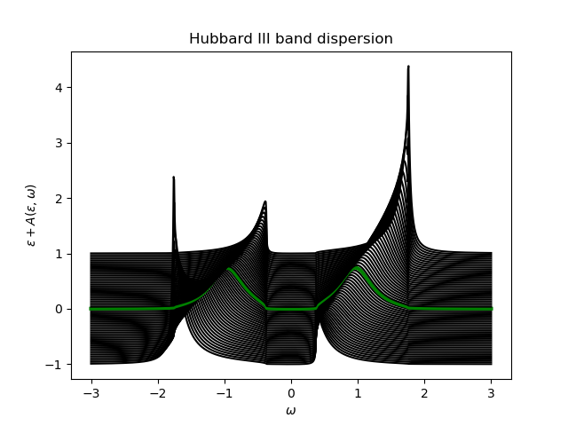
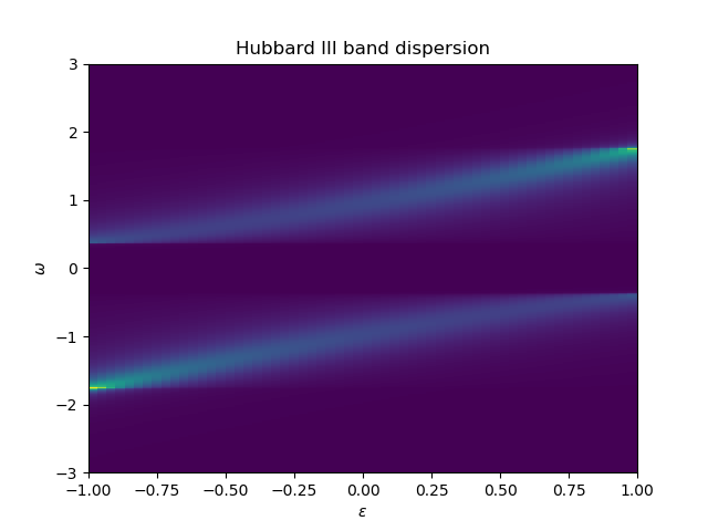
The Band Dispersion

eps_k = np.linspace(-1, 1, 61)
lat_gf = 1 / (np.add.outer(-eps_k, w + 8e-2j) - U**2 / 4 / g0_1)
Aw = -lat_gf.imag / np.pi

plot_band_dispersion(w, Aw, 'Hubbard III band dispersion', eps_k)

• 
• 

Total running time of the script: ( 0 minutes 0.586 seconds)